---------- ---------- ---------- ---------- ---------- ---------- ---------- ----------
Taylor polynomial
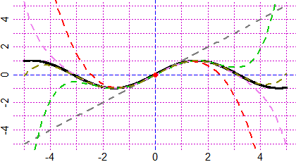 f <- function(x) sin(x); taylor(f, 0, -5,5, -5,5)
# You get the graph of sin and, as you CLICK the screen, Taylor polynomial graphs
# (in 0) up to grade 10. Finally you get:
# 0 , 1 , 0 / 2 , -1 / 6 , 0 / 24 , 1 / 120 , 0 / 720
# -1 / 5040 , 0 / 40320 , 1 / 362880 , 0 / 3628800
# that is, the coefficients of the polynomial, from grade 0 to grade 10.
# If you want to see the function and the the derivatives:
Fx; F1x; F2x; F10x
# sin(x) cos(x) -sin(x) -sin(x)
# If you only want to see the graphs up to a certain degree, press the ESC key.
# I can deduce that around 0:
# sin(x) = x - 1/6*x^3 + 1/120*x^5 - 1/5040*x^7 + 1/362880*x^9 + ģ
#
# log in 1
g <- function(x) log(x); taylor(g, 1, 0,4, -4,3)
f <- function(x) sin(x); taylor(f, 0, -5,5, -5,5)
# You get the graph of sin and, as you CLICK the screen, Taylor polynomial graphs
# (in 0) up to grade 10. Finally you get:
# 0 , 1 , 0 / 2 , -1 / 6 , 0 / 24 , 1 / 120 , 0 / 720
# -1 / 5040 , 0 / 40320 , 1 / 362880 , 0 / 3628800
# that is, the coefficients of the polynomial, from grade 0 to grade 10.
# If you want to see the function and the the derivatives:
Fx; F1x; F2x; F10x
# sin(x) cos(x) -sin(x) -sin(x)
# If you only want to see the graphs up to a certain degree, press the ESC key.
# I can deduce that around 0:
# sin(x) = x - 1/6*x^3 + 1/120*x^5 - 1/5040*x^7 + 1/362880*x^9 + ģ
#
# log in 1
g <- function(x) log(x); taylor(g, 1, 0,4, -4,3)
 # 0 , 1 , -1 / 2 , 2 / 6 , -6 / 24 , 24 / 120 , -120 / 720
# 720 / 5040 , -5040 / 40320 , 40320 / 362880 , -362880 / 3628800
# I can simplify. I put fraction(c()) and paste in "()" the previous rows:
fraction(c(0 , 1 , -1 / 2 , 2 / 6 , -6 / 24 , 24 / 120 , -120 / 720))
# 0 1 -1/2 1/3 -1/4 1/5 -1/6
fraction(c(720 / 5040 , -5040 / 40320 , 40320 / 362880 , -362880 / 3628800))
# 1/7 -1/8 1/9 -1/10
# I can deduce that around 1:
# log(x) = x-1 - (x-1)^2*1/2 + (x-1)^3*1/3 - (x-1)^4*1/4 + (x-1)^5*1/5 + ģ
#
# cos in 0
h <- function(x) cos(x); taylor(h, 0, -4,4, -2,2)
# 0 , 1 , -1 / 2 , 2 / 6 , -6 / 24 , 24 / 120 , -120 / 720
# 720 / 5040 , -5040 / 40320 , 40320 / 362880 , -362880 / 3628800
# I can simplify. I put fraction(c()) and paste in "()" the previous rows:
fraction(c(0 , 1 , -1 / 2 , 2 / 6 , -6 / 24 , 24 / 120 , -120 / 720))
# 0 1 -1/2 1/3 -1/4 1/5 -1/6
fraction(c(720 / 5040 , -5040 / 40320 , 40320 / 362880 , -362880 / 3628800))
# 1/7 -1/8 1/9 -1/10
# I can deduce that around 1:
# log(x) = x-1 - (x-1)^2*1/2 + (x-1)^3*1/3 - (x-1)^4*1/4 + (x-1)^5*1/5 + ģ
#
# cos in 0
h <- function(x) cos(x); taylor(h, 0, -4,4, -2,2)
 # cos(x) = 1 - 1/2*x^2 + 1/24*x^4 - 1/720*x^6 + 1/40320*x^8 - 1/3628800*x^10
#
# exp in 0
k <- function(x) exp(x); taylor(k, 0, -6,5, -3,15)
# cos(x) = 1 - 1/2*x^2 + 1/24*x^4 - 1/720*x^6 + 1/40320*x^8 - 1/3628800*x^10
#
# exp in 0
k <- function(x) exp(x); taylor(k, 0, -6,5, -3,15)
 # exp(x) = 1 + x + x^2/2 + x^3/6 + x^4/24 + x^5/120 + ...
Other examples of use
# exp(x) = 1 + x + x^2/2 + x^3/6 + x^4/24 + x^5/120 + ...
Other examples of use