---------- ---------- ---------- ---------- ---------- ---------- ---------- ----------
# Let's calculate the area of the circle sector depicted below on the left
BF=3; HF=3
PLANE(0,5,0,5)
f=function(x) sqrt(25-x^2); g=function(x) 3/4*x
graph1(f,-5,5,"blue"); graph1(g,-5,5,"blue")
graph(f,4,5,"red"); graph(g,0,4,"red"); segm(0,0, 5,0, "red")
# This is the figure. It is a circle segment. I can take the circle area multiplied by
# the ratio between the angle of the segment and 360°:
A=c(5,0); B=c(0,0); C=c(4,3); angle(A,B,C)
# 36.8699
pi*5^2*angle(A,B,C)/360
# 8.043764 This is the searched area
# Alternatively, I calculate the area of the triangle and that of the remaining part
# where the figure is broken by the vertical segment falling from (4,3)
polyl(c(4,4),c(0,3),"blue")
# The area of the triangle plus the integral of f between 4 and 5:
4*3/2 + integral(f,4,5)
# 8.043764
 # Let's calculate the area of the figure above, in the center:
PLANE(0,1, 0,1)
f=function(x) x^2; g=function(x) x
graph(f,0,1, "blue"); graph(g,0,1,"red")
# The difference between the area under the graph of g and the one below that of f:
integral(g,0,1)-integral(f,0,1)
# 0.1666667
# Or:
h = function(x) g(x)-h(x); integral(h,0,1)
# 0.1666667 which is equivalent to:
fraction(integral(h,0,1))
# 1/6 This is the searched area
#
# The area of the figure above, on the right, between the two curves:
PLANE(0,4,-2,2)
f = function(x) sin(x); g = function(x) (x-2)^2
graph(f,0,4, "red"); graph(g,0,4, "blue")
solution2(f,g,1,2)
# 1.064761
solution2(f,g,2,3)
# 2.67242
h = function(x) f(x)-g(x)
integral(h, solution2(f,g,1,2), solution2(f,g,2,3))
# 1.002636 This is the searched area
# just over a "square"
#
# How to calculate areas enclosed by polar curves.
# Let's calculate the area of the figure above, in the center:
PLANE(0,1, 0,1)
f=function(x) x^2; g=function(x) x
graph(f,0,1, "blue"); graph(g,0,1,"red")
# The difference between the area under the graph of g and the one below that of f:
integral(g,0,1)-integral(f,0,1)
# 0.1666667
# Or:
h = function(x) g(x)-h(x); integral(h,0,1)
# 0.1666667 which is equivalent to:
fraction(integral(h,0,1))
# 1/6 This is the searched area
#
# The area of the figure above, on the right, between the two curves:
PLANE(0,4,-2,2)
f = function(x) sin(x); g = function(x) (x-2)^2
graph(f,0,4, "red"); graph(g,0,4, "blue")
solution2(f,g,1,2)
# 1.064761
solution2(f,g,2,3)
# 2.67242
h = function(x) f(x)-g(x)
integral(h, solution2(f,g,1,2), solution2(f,g,2,3))
# 1.002636 This is the searched area
# just over a "square"
#
# How to calculate areas enclosed by polar curves.

 # In the case of a circle of radius R I have that area A is pi*R^2.
# Generalizing, if R=R(t):
# In the case of a circle of radius R I have that area A is pi*R^2.
# Generalizing, if R=R(t):
 # If the angle t changes from H to K:
# RR = function(t) R(t)^2; A = integral(RR, H,K)/2
# First example: cardioid. Numerically we have:
R = function(t) 1-sin(t); PLANE(-2,2, -3,1); polar(R, 0,2*pi, "blue")
areaPolar(R,0,2*pi,1000) # 4.712327
areaPolar(R,0,2*pi,2000) # 4.712373
areaPolar(R,0,2*pi,4000) # 4.712385
areaPolar(R,0,2*pi,8000) # 4.712388
areaPolar(R,0,2*pi,16000) # 4.712389
# With integration:
R=function(t) 1-sin(t); RR=function(t) R(t)^2; A=integral(RR, 0,2*pi)/2; A
# 4.712389
A/pi
# 1.5 A = 3/2*pi
#
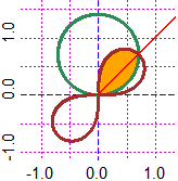
# Second example: the figure above right.
PLANE(-1.25,1.25, -1,1.5)
R1 = function(t) sqrt(2)*sin(t); R2 = function(t) sqrt(sin(2*t))
polar(R1,0,2*pi, "seagreen"); polar(R2,0,2*pi, "brown")
# I give color to the figure:
P=function(x,y) {r=sqrt(x^2+y^2); t=dirArrow1(0,0, x,y)*pi/180; r<=sqrt(sin(t*2)) & r<=sqrt(2)*sin(t)}
for(i in 1:8) FIGURE(P,0,1,0,1, "orange")
polar(R1,0,2*pi, "seagreen"); polar(R2,0,2*pi, "brown")
g = function(x) x; graph1(g, 0,2, "red")
polar(R1,0,pi/4, "blue"); polar(R2,pi/4,pi/2, "red")
# If the angle t changes from H to K:
# RR = function(t) R(t)^2; A = integral(RR, H,K)/2
# First example: cardioid. Numerically we have:
R = function(t) 1-sin(t); PLANE(-2,2, -3,1); polar(R, 0,2*pi, "blue")
areaPolar(R,0,2*pi,1000) # 4.712327
areaPolar(R,0,2*pi,2000) # 4.712373
areaPolar(R,0,2*pi,4000) # 4.712385
areaPolar(R,0,2*pi,8000) # 4.712388
areaPolar(R,0,2*pi,16000) # 4.712389
# With integration:
R=function(t) 1-sin(t); RR=function(t) R(t)^2; A=integral(RR, 0,2*pi)/2; A
# 4.712389
A/pi
# 1.5 A = 3/2*pi
#
# Second example: the figure above right.
PLANE(-1.25,1.25, -1,1.5)
R1 = function(t) sqrt(2)*sin(t); R2 = function(t) sqrt(sin(2*t))
polar(R1,0,2*pi, "seagreen"); polar(R2,0,2*pi, "brown")
# I give color to the figure:
P=function(x,y) {r=sqrt(x^2+y^2); t=dirArrow1(0,0, x,y)*pi/180; r<=sqrt(sin(t*2)) & r<=sqrt(2)*sin(t)}
for(i in 1:8) FIGURE(P,0,1,0,1, "orange")
polar(R1,0,2*pi, "seagreen"); polar(R2,0,2*pi, "brown")
g = function(x) x; graph1(g, 0,2, "red")
polar(R1,0,pi/4, "blue"); polar(R2,pi/4,pi/2, "red")
 R = function(t) ifelse(t < pi/4,R1(t),R2(t)); RR=function(t) R(t)^2; A=integral(RR,0,pi/2)/2; A
# 0.3926991
A/pi
# 0.25
pi/8
# 0.3926991
#
# Another example: the lazy eight ( ρ = √|cos(2θ| ):
R = function(t) ifelse(t < pi/4,R1(t),R2(t)); RR=function(t) R(t)^2; A=integral(RR,0,pi/2)/2; A
# 0.3926991
A/pi
# 0.25
pi/8
# 0.3926991
#
# Another example: the lazy eight ( ρ = √|cos(2θ| ):
 # ( in the right figure θ is in [-π/4,π/4] and in [π-π/4,π+π/4] )
R = function(t) sqrt(abs(cos(2*t))); PLANE(-1.5,1.5, -1.5,1.5); polar(R, 0,2*pi, "blue")
RR=function(t) R(t)^2; A=integral(RR,0,2*pi)/2; A
# 2
# ( in the right figure θ is in [-π/4,π/4] and in [π-π/4,π+π/4] )
R = function(t) sqrt(abs(cos(2*t))); PLANE(-1.5,1.5, -1.5,1.5); polar(R, 0,2*pi, "blue")
RR=function(t) R(t)^2; A=integral(RR,0,2*pi)/2; A
# 2