---------- ---------- ---------- ---------- ---------- ---------- ---------- ----------
Second-order differential equations
# It is convenient to use WolframAlpha to find the solutions, and then R to plot their
# charts. In any case, with R I can check the solutions.
#
# A car that is moving with a constant acceleration of 5 m/s^2 and has a speed of 1 m/s
# at a time when it is 2 m from a reference point.
# With WolframAlpha: f"(x)=5, f'(0)=1, f(0)=2
# I obtain: f(x) = 5*x^2/2+x+2. The graph with R:
f = function(x) 5*x^2/2+x+2; graphF(f, 0,20, "brown")
 # The check
df = function(x) eval(deriv(f,"x"))
deriv2(f,"x"); df(0); f(0)
# 5 1 2
#
# Second example. x = time, y = position of an object of mass m subjected to force
# -k*y by a spring, with k = 4, m = 1. F = m*y"(t) -> y"(x) = -4/1*y(x).
# With WolframAlpha. I obtain y(x) = c2*sin(2*x)+c1*cos(2*x).
# If I put y"(x) = -4*y(x), y(0)=2, y'(0)=0 I obtain: y(x) = 2*cos(2*x) and the graphs:
# The check
df = function(x) eval(deriv(f,"x"))
deriv2(f,"x"); df(0); f(0)
# 5 1 2
#
# Second example. x = time, y = position of an object of mass m subjected to force
# -k*y by a spring, with k = 4, m = 1. F = m*y"(t) -> y"(x) = -4/1*y(x).
# With WolframAlpha. I obtain y(x) = c2*sin(2*x)+c1*cos(2*x).
# If I put y"(x) = -4*y(x), y(0)=2, y'(0)=0 I obtain: y(x) = 2*cos(2*x) and the graphs:
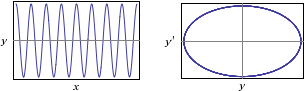 # The check with R
f = function(x) 2*cos(2*x)
df = function(x) eval(deriv(f,"x")); d2f = function(x) eval(deriv2(f,"x"))
F = function(x) d2f(x)+4*f(x); x=1:5; F(x)
# 0 0 0 0 0
f(0); df(0)
# 2 0
# The graph with R:
graph2F(f, 0,20, "brown")
# The check with R
f = function(x) 2*cos(2*x)
df = function(x) eval(deriv(f,"x")); d2f = function(x) eval(deriv2(f,"x"))
F = function(x) d2f(x)+4*f(x); x=1:5; F(x)
# 0 0 0 0 0
f(0); df(0)
# 2 0
# The graph with R:
graph2F(f, 0,20, "brown")
 # Or:
TICKx=pi/2; TICKy=1/2; Plane2(0,20, -2,2)
graph2(f, 0,20, "brown")
underY(-1,-1); underY(1,1); underY(-2,-2); underY(2,2); underY(0,0)
underX(bquote(2*pi),2*pi); underX(bquote(4*pi),4*pi); underX(bquote(6*pi),6*pi)
underX(0,0)
# Or:
TICKx=pi/2; TICKy=1/2; Plane2(0,20, -2,2)
graph2(f, 0,20, "brown")
underY(-1,-1); underY(1,1); underY(-2,-2); underY(2,2); underY(0,0)
underX(bquote(2*pi),2*pi); underX(bquote(4*pi),4*pi); underX(bquote(6*pi),6*pi)
underX(0,0)
 #
# How to trace the phase curve, ie the curve (y(x),y'(x)) [the relationship between
# "y" and its "speed"]?
df = function(x) eval(deriv(f,"x"))
# Where does df change?
x=seq(0,20,0.1); c(min(df(x)),max(df(x)))
# -3.999647 3.999961
Plane(-2,2, -4,4)
param(f,df, 0,20, "brown")
#
# How to trace the phase curve, ie the curve (y(x),y'(x)) [the relationship between
# "y" and its "speed"]?
df = function(x) eval(deriv(f,"x"))
# Where does df change?
x=seq(0,20,0.1); c(min(df(x)),max(df(x)))
# -3.999647 3.999961
Plane(-2,2, -4,4)
param(f,df, 0,20, "brown")
 # In this case, as a phase diagram I get an ellipse: the solution is periodic
#
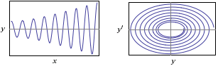
# Third example. Forced oscillations, with external oscillating force F·cos(Ω·t):
# y" = -(k/m)·y + F/m·cos(Ω·t). Consider the following case: F=1, Ω=2
# and the other data as above: y"(x)=-4*y(x)+cos(2*x), y(0)=2, y'(0)=0
# With WolframAlpha I obtain 2*cos(2*x)+1/4*x*sin(2*x) and the graphs:
# In this case, as a phase diagram I get an ellipse: the solution is periodic
#
# Third example. Forced oscillations, with external oscillating force F·cos(Ω·t):
# y" = -(k/m)·y + F/m·cos(Ω·t). Consider the following case: F=1, Ω=2
# and the other data as above: y"(x)=-4*y(x)+cos(2*x), y(0)=2, y'(0)=0
# With WolframAlpha I obtain 2*cos(2*x)+1/4*x*sin(2*x) and the graphs:
 # The check with R
f = function(x) 2*cos(2*x)+1/4*x*sin(2*x)
df = function(x) eval(deriv(f,"x")); d2f = function(x) eval(deriv2(f,"x"))
F = function(x) d2f(x)+4*f(x)-cos(2*x); x=1:5; F(x)
# -6.106227e-16 1.110223e-16 3.330669e-16 1.110223e-16 -1.110223e-16 Practically 0
f(0); df(0)
# 2 0
# The graph:
graph2F(f, 0,30, "brown")
# The check with R
f = function(x) 2*cos(2*x)+1/4*x*sin(2*x)
df = function(x) eval(deriv(f,"x")); d2f = function(x) eval(deriv2(f,"x"))
F = function(x) d2f(x)+4*f(x)-cos(2*x); x=1:5; F(x)
# -6.106227e-16 1.110223e-16 3.330669e-16 1.110223e-16 -1.110223e-16 Practically 0
f(0); df(0)
# 2 0
# The graph:
graph2F(f, 0,30, "brown")
 # The phase curve
df = function(x) eval(deriv(f,"x"))
# Where does df change?
x=seq(0,30,0.1); c(min(df(x)),max(df(x)))
# -15.30207 14.49992
Plane(-8,8, -15,15); param(f,df, 0,30, "brown")
# The phase curve
df = function(x) eval(deriv(f,"x"))
# Where does df change?
x=seq(0,30,0.1); c(min(df(x)),max(df(x)))
# -15.30207 14.49992
Plane(-8,8, -15,15); param(f,df, 0,30, "brown")
 # For these values of F and Ω there is the phenomenon of resonance (oscillations
# increase in amplitude).
#
# Fourth example. Damped oscillations, with y" = -(k/m)·y - k1·y' (with frictional
# force proportional to speed). Example with k1 = 1
# y"(x) = -4*y(x)-y'(x), y(0)=1, y'(0)=3
# With WolframAlpha::
# y(x) = 1/15*exp(-x/2)*(7*sqrt(15)*sin((sqrt(15)*x)/2)+15*cos((sqrt(15)*x)/2))
# For these values of F and Ω there is the phenomenon of resonance (oscillations
# increase in amplitude).
#
# Fourth example. Damped oscillations, with y" = -(k/m)·y - k1·y' (with frictional
# force proportional to speed). Example with k1 = 1
# y"(x) = -4*y(x)-y'(x), y(0)=1, y'(0)=3
# With WolframAlpha::
# y(x) = 1/15*exp(-x/2)*(7*sqrt(15)*sin((sqrt(15)*x)/2)+15*cos((sqrt(15)*x)/2))
 # With R:
S = sqrt(15)
f = function(x) 1/15*exp(-x/2)*(7*S*sin((S*x)/2)+15*cos((S*x)/2))
graph2F(f, 0,20, "brown")
df = function(x) eval(deriv(f,"x"))
x=seq(0, 20, 0.1); c(min(df(x)),max(df(x)))
# -2.307363 3.000000
Plane(-1,2, -3,3); para(f,df, 0,20, "brown")
# With R:
S = sqrt(15)
f = function(x) 1/15*exp(-x/2)*(7*S*sin((S*x)/2)+15*cos((S*x)/2))
graph2F(f, 0,20, "brown")
df = function(x) eval(deriv(f,"x"))
x=seq(0, 20, 0.1); c(min(df(x)),max(df(x)))
# -2.307363 3.000000
Plane(-1,2, -3,3); para(f,df, 0,20, "brown")
 Other examples of use