source("http://macosa.dima.unige.it/r.R") # If I have not already loaded the library
---------- ---------- ---------- ---------- ---------- ---------- ---------- ----------
#
# If we want approximate points with a curve y = A·exp(B·x) we can use regression1
# after transforming y-coordinates by the logarithmic function. An example.
x=c(2.5,7.5,12.5,17.5,22.5,27.5,32.5,37.5,42.5,47.5,52.5,57.5,62.5,67.5,72.5,77.5)
y=c(735,505, 306, 187, 114, 61, 37, 19, 10, 8, 9, 5, 1, 1, 2, 1)/10000
range(x); range(y)
# 2.5 77.5 0.0001 0.0735
Plane(0,90, 0,0.1); Point(x,y, "red"); A=recordPlot()
# the 1st graph
# y=a*exp(b*x) -> log(y) = log(a)+b*x
y1=log(y); range(y1)
# -9.21034 -2.61047
Plane(0,90, -10,0); Point(x,y1, "red")
regression1(x,y1)
# -0.09342 * x + -2.469
g = function(x) -0.09342 * x + -2.469; graph1(g, 0,100, "brown")
# the 2nd graph
a = exp(-2.469); b=-0.09342; a
# 0.08466949
dev.new(width=BF,height=HF); replayPlot(A)
u = function(x) a*exp(b*x); graph1(u,0,100, "blue")
# the 3rd graph [ y = 0.085*exp(-0.093*x) o: y = 0.09*exp(-0.09*x) ]
 # If we look for a curve y = A·exp(B·x) + C we can use F_RUN3. (see)
# If we want, we cau use F_RUN2 also for the curve y = A·exp(B·x):
Plane(0,90, 0,0.1); Point(x,y, "red")
yy2 = function(U,V,x) U*exp(V*x); Fun = function(x) U0*exp(V0*x)
# try:
q = function(x) 0.1*exp(-1*x); graph1(q, 0,100, "seagreen")
q = function(x) 0.1*exp(-0.5*x); graph1(q, 0,100, "seagreen")
q = function(x) 0.1*exp(-0.2*x); graph1(q, 0,100, "seagreen")
# I can choose the parameters
dif=1e300
m1=0.06; M1=0.1; m2=-0.2; M2=0; F_RUN2(x,y,2e5); cat(U0,V0," d:",NUMBER(dif^0.5),"\n")
# 0.09463897 -0.09193754 d: 0.00427094921812952
m1=0.07; M1=0.1; m2=-0.2; M2=0; F_RUN2(x,y,2e5); cat(U0,V0," d:",NUMBER(dif^0.5),"\n")
# 0.09455857 -0.09174792 d: 0.00426937043013651
m1=0.093; M1=0.95; m2=-0.092; M2=-0.09; F_RUN2(x,y,2e5); cat(U0,V0," d:",NUMBER(dif^0.5),"\n")
# 0.09449952 -0.09169488 d: 0.00426928092866325
# y = 0.0945*exp(-0.0917*x) [ o: y = 0.09*exp(-0.09*x) ]
graph1(Fun, 0,100, "brown")
# If we look for a curve y = A·exp(B·x) + C we can use F_RUN3. (see)
# If we want, we cau use F_RUN2 also for the curve y = A·exp(B·x):
Plane(0,90, 0,0.1); Point(x,y, "red")
yy2 = function(U,V,x) U*exp(V*x); Fun = function(x) U0*exp(V0*x)
# try:
q = function(x) 0.1*exp(-1*x); graph1(q, 0,100, "seagreen")
q = function(x) 0.1*exp(-0.5*x); graph1(q, 0,100, "seagreen")
q = function(x) 0.1*exp(-0.2*x); graph1(q, 0,100, "seagreen")
# I can choose the parameters
dif=1e300
m1=0.06; M1=0.1; m2=-0.2; M2=0; F_RUN2(x,y,2e5); cat(U0,V0," d:",NUMBER(dif^0.5),"\n")
# 0.09463897 -0.09193754 d: 0.00427094921812952
m1=0.07; M1=0.1; m2=-0.2; M2=0; F_RUN2(x,y,2e5); cat(U0,V0," d:",NUMBER(dif^0.5),"\n")
# 0.09455857 -0.09174792 d: 0.00426937043013651
m1=0.093; M1=0.95; m2=-0.092; M2=-0.09; F_RUN2(x,y,2e5); cat(U0,V0," d:",NUMBER(dif^0.5),"\n")
# 0.09449952 -0.09169488 d: 0.00426928092866325
# y = 0.0945*exp(-0.0917*x) [ o: y = 0.09*exp(-0.09*x) ]
graph1(Fun, 0,100, "brown")
 #
# If I have the points that have the following coordinates: bilog.htm and I know that
# they are of the graph of a polynomial function, I can find the degree of it if I
# transform x and y coordinates by the logarithmic function. I can copy the file to the
# clipboard and then with
dati = read.table("clipboard",sep=",")
dim(dati)
# 21 2
x=dati$V1; y=dati$V2
# or I can use bi_log.htm
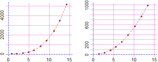
min(x); max(x); min(y); max(y)
# -1 15 1.2153e-10 6080
BF=4; HF=3
Plane(-1,15, 0,6100)
Point(x,y, "blue")
# I have the graph below left
#
# If I have the points that have the following coordinates: bilog.htm and I know that
# they are of the graph of a polynomial function, I can find the degree of it if I
# transform x and y coordinates by the logarithmic function. I can copy the file to the
# clipboard and then with
dati = read.table("clipboard",sep=",")
dim(dati)
# 21 2
x=dati$V1; y=dati$V2
# or I can use bi_log.htm
min(x); max(x); min(y); max(y)
# -1 15 1.2153e-10 6080
BF=4; HF=3
Plane(-1,15, 0,6100)
Point(x,y, "blue")
# I have the graph below left

# To transform the data with the logarithmic scales, I add
# two constants in order to obtain positive coordinates.
x1=x+1.5; y1=y+1
min(x1); max(x1); min(y1); max(y1)
#  0.5  16.5  1  6081
Plane(0,17, 0,6100); Point(x1,y1, "blue") |  |
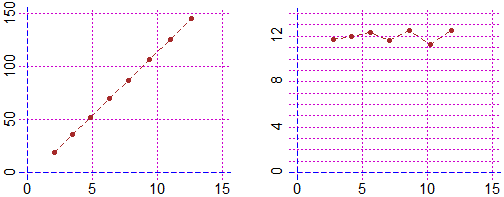
# Having obtained the graph on the right, I transform it using logarithmic function;
# I get the graph above in the middle.
x2=log(x1); y2=log(y1)
min(x2); max(x2); min(y2); max(y2)
# -0.6931472 2.80336 1.215299e-10 8.712924
Plane(-1,3, 0,9); Point(x2,y2, "blue")
# I understand that the function tends to have slope 3, ie that the polynomial
# function has degree 3. I can verify this by calculating the slopes:
for(i in 1:20) print((y2[i+1]-y2[i])/(x2[i+1]-x2[i]))
# 1.851189 ... 3.520021 3.486567 3.457125 3.431019
# Now I can find the function with regression3:
regression3(x,y)
# 2 * x^3 + -3 * x^2 + -1.76e-11 * x + 5
f = function(x) 2 * x^3 + -3 * x^2 + 5
Plane(-1,15, 0,6100); Point(x,y, "blue")
graph1(f, -1,15, "brown")
# I get the graph above right.
#
# The polynomial trend data can also be studied through successive passages to the
# slope graph. If N passages are used to arrive at points with approximately rectilinear
# trends, this means that the data had approximately polynomial trend of degree N+1.
# See here for an example:
 Other examples of use