---------- ---------- ---------- ---------- ---------- ---------- ---------- ----------
R. 1. Start use (more)
Introduction Use as calculator Other calculi Figures Graphs Statistics More
This guide is just an introduction to the main commands, to get confident with the
software and to illustrate some of the activities that can be faced with it from the
basic school (it is useful for teachers in order to prepare materials and in some cases
to propose things to be done to students after they have learned to do similar things
"by hand"). At the bottom there is an index (for other indexes see here).
# (A) At startup, the program has a line beginning with >. After this symbol I can
# type an "input", followed by "enter key", and get a possible "output", written in
# blue, preceded by [1]. With some "commands" I can have more lines of output; in
# these cases the following lines are preceded by [2], [3], ... A simple example:
> 10/4
# [1] 2.5
# In the examples we will do we will not put > so that the commands can be copied from
# here and put directly into R
# The parts that follow # (like these) are for those who read; they can be copied to R
# without giving rise to any execution: in R the texts preceded by # are just comments.
# You can change size and style of the font, and other aspects (for example, to use the
# projector): see.
# To use many commands (indicated by point (C) down) you must first write to R (only
# once) the following line. You should copy it and paste it immediately:
source("http://macosa.dima.unige.it/r.R")
USE as CALCULATOR
# (B) R can be used as an excellent calculator; the division is "/", the multiplication
# "*", a power elevation, such as 6 to 2, is indicated by 6^2, where "^" indicates that
# the 2 should be thought as if it was raised.
6+2
# [1] 8
6-2; 2-6; 6*2; 6/2; 6^2
# [1] 4
# [1] -4
# [1] 12
# [1] 3
# [1] 36
# As you have seen, I can run multiple commands separated by ;. I get the results
# one below the other.
# The results can have many or infinite digits; only a few are shown:
5000/12
# [1] 416.6667
# 5000/12 results 416.66666 ... but the program displays only 7 digits rounding the
# final figure: 416.66666... -> 416.6667 (it is closer to 5000/12 than 416.6666).
# (C) In addition to + * / ... with R you can calculate the values of other functions,
# which relate outputs to inputs. Generally the inputs are enclosed in brackets. Some
# examples, round, sqrt or rad2, rad3:
round(5000/12, 3); round(5000/12, 1); round(5000/12, 0); round(5000/12, -2)
# [1] 416.667
# [1] 416.7
# [1] 417
# [1] 400
# round(5000/12, 3) rounds to the 3rd digit after ".", round(5000/12, 1) to 1st digit,
# round(5000/12, 0) to integers, rounds(5000/12, -2) to hundreds. For example, if I
# have a cost of 5000 euros to divide between 12 people I calculate 5000/12, rounding
# the result to the cents, that is to the 2nd digit after ".":
round(5000/12, 2)
# [1] 416.67
sqrt(4); sqrt(3); sqrt(3)^2
# [1] 2
# [1] 1.732051
# [1] 3
# sqrt acts for "square root". The side of a square that must have the area of 3 m^2
# must be 1.73 m, ie 173 cm.
# Instead of sqrt you can use rad2. You can use rad3 to calculate the cubic root.
# The side (in cm) of a volume cube of 500 cm^3 (half liter):
rad3(500)
# [1] 7.937005
# (D) For fractional calculations and to represent finite or periodic numbers in the
# form of fractions it may be useful the command fraction (or "frazio"). Examples:
fraction(1.3333333333333); fraction(0.125); fraction(10/4); fraction(15/60+1/2)
# 4/3 1/8 5/2 3/4
# To get a ratio in percentage form, eg 23/54 as 42.6% or 43%, I do:
23/54*100; round(23/54*100,1); round(23/54*100,0)
# 42.59259 42.6 43
# To write large or small numbers you can use the so-called exponential notation, as
# you do with the calculator, using eg e3 to mean a multiplication for 10^3 and e-3 to
# mean a division for 10^3, ie a multiplication for 10^-3.
# R uses the same notation to indicate large and small numbers.
# Here are some ways to write 100 thousand and 2 tenths of a thousand:
100000; 100*1000; 100e3; 0.0002; 2e-4
# 1e+05 1e+05 1e+05 2e-04 2e-04
# If you have to calculate 15+27 and divide the result by twice the sum of 36 and 25,
# ie calculate what at school is sometimes written (12+27)/[2*(36+25)], you need to be
# careful: in math the parentheses have different meanings than those given at school:
# square brackets, [ and ],and braces, { and }, are used to indicate particular
# mathematical objects. Software, and mathematicians, write a term like the previous
# using only round parentheses: (12+27)/(2*(36+25)). They eventually change the size:
# (12+27)/(2*(36+25)). Using R you can improve readability by adding white spaces:
(12+27) / ( 2*(36+25) )
# [1] 0.3196721
# In fact, I can put all the spaces I want between brackets, numbers, and operations.
# (E) Here is how to perform the division with the rest between two integers and how
# to list the positive integers for which an integer can be divisible (its divisors).
div(13, 4)
# [1] 3 1
# 3 con resto 1; infatti 13 = 4*3 + 1
divisors(12) # or: divisori(12)
# [1] 1 2 3 4 6 12
Other CALCULI
# (F) In a formula like area = length*width (area of the rectangle) area, length and
# width are variables, ie the names to which values can be replaced. Also in R I can
# use variables. I have to be careful about the size of the letters: Width, WIDTH and
# width are three different variables. Example:
length = 10; width = 5
length*width
# [1] 50
length*Width
# Error: "Width" not found
# I could also put the result of length*width into another variable and then look
# for the value of it:
area = length*width
area
# [1] 50
# (G) If I have to do the same calculation referring to several numbers, such as 5, 10
# and 3, I can put these into a collection of numbers, ie put them in c(5,10,3) and
# make calculations with this new object:
c(5,10,3)*2
# [1] 10 20 6
# There are also calculations that are made specifically on the collections of objects;
# eg If I want to sort the data I put them as input of the sort function and get the
# output as data in ascending order:
sort( c(5,10,3) )
# [1] 3 5 10
# I can extract a number from a collection by pointing - between [ and ] - the place:
joe = c(5,10,3); joe[1]; joe[2]
# [1] 5
# [1] 10
# Let's see an example of use. I put in height_pupils the heights in cm of some pupils
# of a class (I use "_" to combine "height" and "pupils" in one variable, but I could
# use eg HeightPupils). Then I put them in order:
height_pupils = c(118, 135, 127, 119, 121, 124, 130, 132, 128, 122, 121, 123, 127)
sort(height_pupils)
# [1] 118 119 121 121 122 123 124 127 127 128 130 132 135
# Other calculations I can do (we see the outputs immediately):
data = height_pupils; min(data); max(data); length(data); sum(data)
# [1] 118
# [1] 135
# [1] 13
# [1] 1627
# The meaning of commands is obvious. I copied "height_pupils" into "data" so that I
# had a shorter name to write.
# NOTE If I press the arrow key "up" [^] I see the previous commands again, if I press
# the arrow key "down" [v] I see the subsequent commands: this is convenient for
# recalling or modifying them. Try to use them.
FIGURES
# (H) Let's see some basic commands to build geometric figures. Let's go through
# examples.
PLANE(-1,10, -1,10)
 # A window opens where the left figure appears: a "squared paper" with numbers that
# represent, as in a geographic map, the coordinates of the various points. The point
# whose horizontal and vertical coordinates are 7 and 4 appears red. It was plotted
# with the command:
POINT(7,4, "red")
# The smallest point (blue) was obtained with:
Point(2,4, "blue")
# By moving the mouse over the title bar of the graphics window (see below) I can move
# it. By moving over edges or angles I can resize it (see above on the right).
# A window opens where the left figure appears: a "squared paper" with numbers that
# represent, as in a geographic map, the coordinates of the various points. The point
# whose horizontal and vertical coordinates are 7 and 4 appears red. It was plotted
# with the command:
POINT(7,4, "red")
# The smallest point (blue) was obtained with:
Point(2,4, "blue")
# By moving the mouse over the title bar of the graphics window (see below) I can move
# it. By moving over edges or angles I can resize it (see above on the right).
 # To delete a window I do not need, I click the red button X .
# New "planes" appear in overlapping windows. To see the old ones I can move the new
# windows.
# I can save a picture using Copy from the File menu (In Windows I can also click the
# picture, select "bitmap", then copy it in Paint, modify and save as PNG file, or in a
# word processing tool. In Mac I have to paste it directly in the tool I want to use; I
# can use an application similar to Paint, PaintBrush, which, if it is not already
# installed on your Mac, you can download for free [search on Google "paintbrush"])
# The initial window was wide and high about 3 inches. If I type BF and HF (base and
# height of the window frame) I get:
BF;HF
# [1] 3
# [1] 3
# I can change the size of the window. Example:
BF=4; HF=2; PLANE(-50,50, 0,50)
# To delete a window I do not need, I click the red button X .
# New "planes" appear in overlapping windows. To see the old ones I can move the new
# windows.
# I can save a picture using Copy from the File menu (In Windows I can also click the
# picture, select "bitmap", then copy it in Paint, modify and save as PNG file, or in a
# word processing tool. In Mac I have to paste it directly in the tool I want to use; I
# can use an application similar to Paint, PaintBrush, which, if it is not already
# installed on your Mac, you can download for free [search on Google "paintbrush"])
# The initial window was wide and high about 3 inches. If I type BF and HF (base and
# height of the window frame) I get:
BF;HF
# [1] 3
# [1] 3
# I can change the size of the window. Example:
BF=4; HF=2; PLANE(-50,50, 0,50)
 # If I do not change BF and HF the size remains these. Horizontal coordinates range (at
# least) from -50 to 50. Vertical coordinates range (at least) from 0 to 50. To plot
# the new windows in the original dimensions I type:
BF=3; HF=3
# I write 4,2 to indicate the point having the coordinates 4 and 2. With the following
# commands I draw in blue the circle whose center is 4,2 and radius is 3 and in black
# the center. Then I draw the circle that passes through the 3 points whose first
# coordinates I put in x and the second in y. I draw the circle in red and the points
# in black. Instead of "black" I can use number 1.
PLANE(-1,10, -1,10)
circle(4,2, 3, "blue"); POINT(4,2,"black")
x = c(5, 8, 9); y = c(9, 3, 7.5)
circle3p(x,y, "red"); POINT(x,y, 1)
# If I do not change BF and HF the size remains these. Horizontal coordinates range (at
# least) from -50 to 50. Vertical coordinates range (at least) from 0 to 50. To plot
# the new windows in the original dimensions I type:
BF=3; HF=3
# I write 4,2 to indicate the point having the coordinates 4 and 2. With the following
# commands I draw in blue the circle whose center is 4,2 and radius is 3 and in black
# the center. Then I draw the circle that passes through the 3 points whose first
# coordinates I put in x and the second in y. I draw the circle in red and the points
# in black. Instead of "black" I can use number 1.
PLANE(-1,10, -1,10)
circle(4,2, 3, "blue"); POINT(4,2,"black")
x = c(5, 8, 9); y = c(9, 3, 7.5)
circle3p(x,y, "red"); POINT(x,y, 1)
 # The center of the red circle is also drawn. I got it and the radius as follows:
center3p; radius3p
# [1] 6.076923 5.788462
# [1] 3.387291
POINT(6.076923, 5.788462, "orange")
# Here are some color names [enter Colors() to see others]:
# The center of the red circle is also drawn. I got it and the radius as follows:
center3p; radius3p
# [1] 6.076923 5.788462
# [1] 3.387291
POINT(6.076923, 5.788462, "orange")
# Here are some color names [enter Colors() to see others]:
 # 1 black 2 grey 3 white 4 brown 5 orange 6 red 7 pink
# 8 magenta 9 blue 10 cyan 11 yellow 12 green 13 seagreen
# (I) Let's see some other figure: lines, angles, ...
PLANE(0,10, 0,10)
# I plot a few points (figure on the left):
POINT(1,9,"blue"); POINT(4,9, "blue"); POINT(0,6,"brown"); POINT(4,8, "brown")
POINT(3,5,"magenta"); POINT(7,4, "magenta"); POINT(2,1, "red"); POINT(7,2,"red")
# 1 black 2 grey 3 white 4 brown 5 orange 6 red 7 pink
# 8 magenta 9 blue 10 cyan 11 yellow 12 green 13 seagreen
# (I) Let's see some other figure: lines, angles, ...
PLANE(0,10, 0,10)
# I plot a few points (figure on the left):
POINT(1,9,"blue"); POINT(4,9, "blue"); POINT(0,6,"brown"); POINT(4,8, "brown")
POINT(3,5,"magenta"); POINT(7,4, "magenta"); POINT(2,1, "red"); POINT(7,2,"red")
 # then (on the right) two segments, a halfline and a straight line for two points (the
# latter are only partially traced):
segm(1,9, 4,9, "blue"); segm(0,6, 4,8, "brown")
halfline(3,5, 7,4, "magenta") # the halfline starting from 3,5, passing through 7,4
line2p(2,1, 7,2, "red") # the line passing through 2,1 and 7,2
# Let's see some other simple figure:
# then (on the right) two segments, a halfline and a straight line for two points (the
# latter are only partially traced):
segm(1,9, 4,9, "blue"); segm(0,6, 4,8, "brown")
halfline(3,5, 7,4, "magenta") # the halfline starting from 3,5, passing through 7,4
line2p(2,1, 7,2, "red") # the line passing through 2,1 and 7,2
# Let's see some other simple figure:
 PLANE(0,10, 0,10)
A = c(0,6); B = c(2,10); C = c(5,4)
POINT(A[1],A[2], "blue"); POINT(B[1],B[2], "blue"); POINT(C[1],C[2], "blue")
line(A[1],A[2], B[1],B[2], "blue"); line(A[1],A[2], C[1],C[2], "blue")
# I have plotted points and traced thin segments with the command line (instead of
# segm). I have stored every point (A, B, C) in a variable, as collection - see (G) -
# of his coordinates.
# With point_point I calculate the distance of A from B, with inclination the
# inclination of AB e AC. With angle I can measure the angle CAB directly.
# With SLOPE I calculate the slope of the line of a given inclination.
point_point(A[1],A[2], B[1],B[2])
# [1] 4.472136
inclination(A[1],A[2], B[1],B[2])
# [1] 63.43495
SLOPE(63.43495)
# [1] 2 # (B[2]-A[2])/(B[1]-A[1])
inclination(A[1],A[2], C[1],C[2])
# [1] -21.80141
angle(C,A,B)
# [1] 85.23636
# Then with mid2p I traced the middle point of AB
mid2p(A[1],A[2], B[1],B[2], "red")
# In the figure on the right I traced the axis of AB, ie the line perpendicular to AB
# and passing through its middle point.
perp2p(A[1],A[2], B[1],B[2], "red")
# (J) Let's see how to draw polyline and polygons. With polyline I trace the line
# formed by the segments joining the points with the indicated coordinates. In the
# following example the first point coincides with the last one (in this case the
# polyline is a polygon). leng calculates its length.
PLANE(-3,9,-2,10)
x = c(-3,2,8,8,-3); y = c(1,1,9,-1,1)
polyline(x,y, "blue"); POINT(x,y, "red")
leng(x,y)
# [1] 36.18034
# If I want to calculate the length of the first 3 segments, between 1^ and 4^ points:
leng(x[1:4],y[1:4])
# [1] 25
PLANE(0,10, 0,10)
A = c(0,6); B = c(2,10); C = c(5,4)
POINT(A[1],A[2], "blue"); POINT(B[1],B[2], "blue"); POINT(C[1],C[2], "blue")
line(A[1],A[2], B[1],B[2], "blue"); line(A[1],A[2], C[1],C[2], "blue")
# I have plotted points and traced thin segments with the command line (instead of
# segm). I have stored every point (A, B, C) in a variable, as collection - see (G) -
# of his coordinates.
# With point_point I calculate the distance of A from B, with inclination the
# inclination of AB e AC. With angle I can measure the angle CAB directly.
# With SLOPE I calculate the slope of the line of a given inclination.
point_point(A[1],A[2], B[1],B[2])
# [1] 4.472136
inclination(A[1],A[2], B[1],B[2])
# [1] 63.43495
SLOPE(63.43495)
# [1] 2 # (B[2]-A[2])/(B[1]-A[1])
inclination(A[1],A[2], C[1],C[2])
# [1] -21.80141
angle(C,A,B)
# [1] 85.23636
# Then with mid2p I traced the middle point of AB
mid2p(A[1],A[2], B[1],B[2], "red")
# In the figure on the right I traced the axis of AB, ie the line perpendicular to AB
# and passing through its middle point.
perp2p(A[1],A[2], B[1],B[2], "red")
# (J) Let's see how to draw polyline and polygons. With polyline I trace the line
# formed by the segments joining the points with the indicated coordinates. In the
# following example the first point coincides with the last one (in this case the
# polyline is a polygon). leng calculates its length.
PLANE(-3,9,-2,10)
x = c(-3,2,8,8,-3); y = c(1,1,9,-1,1)
polyline(x,y, "blue"); POINT(x,y, "red")
leng(x,y)
# [1] 36.18034
# If I want to calculate the length of the first 3 segments, between 1^ and 4^ points:
leng(x[1:4],y[1:4])
# [1] 25
 # With polyC I close the polyline by coloring the polygon it delimits.
PLANE(-3,9,-2,10); polyC(x,y,"yellow")
# At the yellow polygon I added a red rectangle, obtained with:
A = c(0,2, 2,0, 0); B = c(4,4, 7,7, 4); polyline(A,B, "red")
----------------------------------------------
# We shall see later how to use PPP(). It can be usefully employed by the teacher in
# the basic school to build animated documents. Two examples:
BF=4; HF=4; PLANE(-5,9,-5,9)
A = function() {PPP(); A1=round(xP); A2=round(yP);
CLEAN(-5,9,-5,9); BOX(); POINT(A1,A2,"brown");
PPP(); B1=round(xP); B2=round(yP); POINT(B1,B2,"brown");
line(A1,A2,B1,B2, "brown"); POINT( (A1+B1)/2,(A2+B2)/2,"seagreen");
cat(A1," ",A2," ",B1," ",B2, " Green point = ?","\n")}
cat("Type A() and click the screen twice. What are the coordinates of the green dot?","\n")
# Type A() and click the screen twice. What are the coordinates of the green dot?
A()
# -1 6 6 2 Green point = ?
# With polyC I close the polyline by coloring the polygon it delimits.
PLANE(-3,9,-2,10); polyC(x,y,"yellow")
# At the yellow polygon I added a red rectangle, obtained with:
A = c(0,2, 2,0, 0); B = c(4,4, 7,7, 4); polyline(A,B, "red")
----------------------------------------------
# We shall see later how to use PPP(). It can be usefully employed by the teacher in
# the basic school to build animated documents. Two examples:
BF=4; HF=4; PLANE(-5,9,-5,9)
A = function() {PPP(); A1=round(xP); A2=round(yP);
CLEAN(-5,9,-5,9); BOX(); POINT(A1,A2,"brown");
PPP(); B1=round(xP); B2=round(yP); POINT(B1,B2,"brown");
line(A1,A2,B1,B2, "brown"); POINT( (A1+B1)/2,(A2+B2)/2,"seagreen");
cat(A1," ",A2," ",B1," ",B2, " Green point = ?","\n")}
cat("Type A() and click the screen twice. What are the coordinates of the green dot?","\n")
# Type A() and click the screen twice. What are the coordinates of the green dot?
A()
# -1 6 6 2 Green point = ?
 BF=4; HF=4; PLANE(0,12,0,12)
S=12; X=3; Y=S/X; polyline(c(0,X,X,0,0),c(0,0,Y,Y,0), "blue"); POINT(X,Y,"red")
A = function() {PPP(); x=round(xP,1); polyline(c(0,X,X,0,0),c(0,0,Y,Y,0), "grey"); POINT(X,Y,"red");
X<<-x; Y<<-S/x; polyline(c(0,X,X,0,0),c(0,0,Y,Y,0), "blue"); POINT(X,Y,"red")}
cat("Type A() and click the screen. Then repeat several times. What do you observe?","\n")
# Type A() and click the screen. Then repeat several times. What do you observe?
A()
...
GRAPHS
# (K) Let's see how to make a graph of a phenomenon that varies with another. Plane
# (with only one uppercase letter, "P") represents the "x" and "y" with scales that
# can be different.
# Example: average consumption of kg of fresh fruit per year by an Italian.
year = c(1880,1890,1900,1910,1920,1930,1940,1950,1960,1970,1980)
fruit = c(19, 21, 23, 28, 31, 27, 23, 37, 65, 88, 79)
# max is useful for choosing the "Plane": I find the maximum is 88, so I change y
# between 0 and 90
max(fruit)
# [1] 88
BF=4; HF=2.5
Plane(1880,1980, 0,90)
polyline(year,fruit, "blue"); POINT(year,fruit,"brown")
BF=4; HF=4; PLANE(0,12,0,12)
S=12; X=3; Y=S/X; polyline(c(0,X,X,0,0),c(0,0,Y,Y,0), "blue"); POINT(X,Y,"red")
A = function() {PPP(); x=round(xP,1); polyline(c(0,X,X,0,0),c(0,0,Y,Y,0), "grey"); POINT(X,Y,"red");
X<<-x; Y<<-S/x; polyline(c(0,X,X,0,0),c(0,0,Y,Y,0), "blue"); POINT(X,Y,"red")}
cat("Type A() and click the screen. Then repeat several times. What do you observe?","\n")
# Type A() and click the screen. Then repeat several times. What do you observe?
A()
...
GRAPHS
# (K) Let's see how to make a graph of a phenomenon that varies with another. Plane
# (with only one uppercase letter, "P") represents the "x" and "y" with scales that
# can be different.
# Example: average consumption of kg of fresh fruit per year by an Italian.
year = c(1880,1890,1900,1910,1920,1930,1940,1950,1960,1970,1980)
fruit = c(19, 21, 23, 28, 31, 27, 23, 37, 65, 88, 79)
# max is useful for choosing the "Plane": I find the maximum is 88, so I change y
# between 0 and 90
max(fruit)
# [1] 88
BF=4; HF=2.5
Plane(1880,1980, 0,90)
polyline(year,fruit, "blue"); POINT(year,fruit,"brown")
 # I also put two inscriptions along the axes with these commands:
abovex("year"); abovey("fruit")
# See here for data entry in tabular form.
# I can also graph the functions in which "x" and "y" are linked by a formula
# Ex: the conversion of the temperature in degrees Celsius to that in Fahrenheit.
# I also put two inscriptions along the axes with these commands:
abovex("year"); abovey("fruit")
# See here for data entry in tabular form.
# I can also graph the functions in which "x" and "y" are linked by a formula
# Ex: the conversion of the temperature in degrees Celsius to that in Fahrenheit.
 Fa = function(Ce) 32 + 72/40*Ce
Fa(-30); Fa(110)
# -22 230
Plane(-30,110, -22,230)
graph(Fa, -30,110, "brown")
abovey("°F"); abovex("°C")
POINT(100,Fa(100),"blue"); POINT(0,Fa(0),"blue")
# I got the chart on top left.
Fa(100)
# [1] 212
# To find the temperature in °F that corresponds to 100°C I simply calculated Fa(100).
# To find what is the temperature k in °C that corresponds to 100°F (see the graph on
# the right) I have to solve the problem: "for which k Fa(k) = 100?". I could do it
# "by hand". Or I can proceed using the solution command as follows:
solution(Fa,100, 20,60)
# [1] 37.77778
# I put Fa,100 because I must find the solution of the problem:
# for what input Fa is worth 100?
# I put 20,60 to indicate two values among which is the solution, derived from the
# graph. 37.777… is therefore the value of k.
# I can proceed in the same way for any other value.
# The computer does nothing but speed up a process that I could do directly with zoom,
# to find more precisely the °C degrees to which it corresponds to 100°F
Fa = function(Ce) 32 + 72/40*Ce
Fa(-30); Fa(110)
# -22 230
Plane(-30,110, -22,230)
graph(Fa, -30,110, "brown")
abovey("°F"); abovex("°C")
POINT(100,Fa(100),"blue"); POINT(0,Fa(0),"blue")
# I got the chart on top left.
Fa(100)
# [1] 212
# To find the temperature in °F that corresponds to 100°C I simply calculated Fa(100).
# To find what is the temperature k in °C that corresponds to 100°F (see the graph on
# the right) I have to solve the problem: "for which k Fa(k) = 100?". I could do it
# "by hand". Or I can proceed using the solution command as follows:
solution(Fa,100, 20,60)
# [1] 37.77778
# I put Fa,100 because I must find the solution of the problem:
# for what input Fa is worth 100?
# I put 20,60 to indicate two values among which is the solution, derived from the
# graph. 37.777… is therefore the value of k.
# I can proceed in the same way for any other value.
# The computer does nothing but speed up a process that I could do directly with zoom,
# to find more precisely the °C degrees to which it corresponds to 100°F
 STATISTICS
# (L) The first statistical calculations, which can be seen from the early years of
# school, are cross histograms. At a later time one can use the square or millimeter
# paper. Only then does it make sense to use the computer, to automate some of the
# process that we have learned to deal with "by hand". Here are some examples.
# The inhabitants (in thousands) of the North, the Center and the South (of Italy);
# the simplest way (bar, strip and pie chart):
N = 25755; C = 12068; S = 20843; Italia = c(N,C,S)
bar(Italia); pieC(Italia); strip(Italia)
# % 43.90107 20.57069 35.52824
STATISTICS
# (L) The first statistical calculations, which can be seen from the early years of
# school, are cross histograms. At a later time one can use the square or millimeter
# paper. Only then does it make sense to use the computer, to automate some of the
# process that we have learned to deal with "by hand". Here are some examples.
# The inhabitants (in thousands) of the North, the Center and the South (of Italy);
# the simplest way (bar, strip and pie chart):
N = 25755; C = 12068; S = 20843; Italia = c(N,C,S)
bar(Italia); pieC(Italia); strip(Italia)
# % 43.90107 20.57069 35.52824
 # If I want, I can give names:
R = c("North","Center","South")
BarNames=R; bar(Italia); PieNames=R; pieC(Italia); StripNames=R; strip(Italia)
# % 43.90107 20.57069 35.52824
North Center South
# Or:
names = c("N","C","S")
BarNames = names; Bar(Italia)
PieNames = names; Pie(Italia)
Strip(Italia)
# yellow,cyan,... % 43.90107 20.57069 35.52824
# yellow,cyan,... N C S
# If I want, I can give names:
R = c("North","Center","South")
BarNames=R; bar(Italia); PieNames=R; pieC(Italia); StripNames=R; strip(Italia)
# % 43.90107 20.57069 35.52824
North Center South
# Or:
names = c("N","C","S")
BarNames = names; Bar(Italia)
PieNames = names; Pie(Italia)
Strip(Italia)
# yellow,cyan,... % 43.90107 20.57069 35.52824
# yellow,cyan,... N C S
 # If I want I can use UNDER(name,x) and ABOVE(name,x) to put names under/above the
# bars; in x I must put the number of the bar. The same example (put 'UNDER("%",0.5)'
# if you want '%' under y-axis):
Bar( c(25755,12068,20843) ); ABOVE(25755,1); ABOVE(12068,2); ABOVE(20843,3)
UNDER("North",1); UNDER("Center",2); UNDER("South",3); UNDER("%",0)
# If I want I can use UNDER(name,x) and ABOVE(name,x) to put names under/above the
# bars; in x I must put the number of the bar. The same example (put 'UNDER("%",0.5)'
# if you want '%' under y-axis):
Bar( c(25755,12068,20843) ); ABOVE(25755,1); ABOVE(12068,2); ABOVE(20843,3)
UNDER("North",1); UNDER("Center",2); UNDER("South",3); UNDER("%",0)
 # I can put names above/under the strip with above(name,x), under(name,x), under2(name,x)
Strip(c(25755,12068,20843)); above("North",21); above("Center",53); above("South",82)
# I can put names above/under the strip with above(name,x), under(name,x), under2(name,x)
Strip(c(25755,12068,20843)); above("North",21); above("Center",53); above("South",82)
 Strip(c(25755,12068,20843)); above(25755,21); above(12068,53); above(20843,82)
under("Italy",25); under2("North-Center-South",25)
Strip(c(25755,12068,20843)); above(25755,21); above(12068,53); above(20843,82)
under("Italy",25); under2("North-Center-South",25)
 # To get rounded percentage distribution - see (C) - I can do:
distribution(Italia, 0)
# 44 21 36
distribution(Italia, 2)
# 43.9 20.57 35.53 # if I want, then I write 43.90 instead of 43.9
distribution(Italia, -1)
# 40 20 40
# (M) These were already classified data. Let's see how to analyze individual data.
# As we see in the following example, we observe that commands can be broken over
# multiple rows. Here are the lengths of many broad beans (ie bean seeds) collected by
# a 12-year-old class. All lines must be copied and pasted, from "beans = c(" to the
# final line )".
beans = c(
1.35,1.65,1.80,1.40,1.65,1.80,1.40,1.65,1.85,1.40,1.65,1.85,1.50,1.65,1.90,
1.50,1.65,1.90,1.50,1.65,1.90,1.50,1.70,1.90,1.50,1.70,1.90,1.50,1.70,2.25,
1.55,1.70,1.55,1.70,1.55,1.70,1.60,1.70,1.60,1.75,1.60,1.75,1.60,1.80,1.60,
1.80,1.60,1.80,1.60,1.80,1.00,1.55,1.70,1.75,1.30,1.55,1.70,1.75,1.40,1.60,
1.70,1.75,1.40,1.60,1.70,1.80,1.40,1.60,1.70,1.80,1.40,1.60,1.70,1.80,1.40,
1.60,1.70,1.80,1.40,1.60,1.70,1.80,1.40,1.60,1.70,1.80,1.40,1.60,1.70,1.80,
1.45,1.60,1.70,1.80,1.50,1.60,1.70,1.80,1.50,1.60,1.70,1.85,1.50,1.60,1.70,
1.85,1.50,1.60,1.75,1.90,1.50,1.60,1.75,1.90,1.50,1.65,1.75,1.90,1.55,1.65,
1.75,1.95,1.55,1.65,1.75,2.00,1.55,1.65,1.75,2.30,1.35,1.65,1.80,1.40,1.65,
1.80,1.40,1.65,1.85,1.40,1.65,1.85,1.50,1.65,1.90,1.50,1.65,1.90,1.50,1.65,
1.90,1.50,1.70,1.90,1.50,1.70,1.90,1.50,1.70,2.25,1.55,1.70,1.55,1.70,1.55,
1.70,1.60,1.70,1.60,1.75,1.60,1.75,1.60,1.80,1.60,1.80,1.60,1.80,1.60,1.80,
1.00,1.55,1.70,1.75,1.30,1.55,1.70,1.75,1.40,1.60,1.70,1.75,1.40,1.60,1.70,
1.80,1.40,1.60,1.70,1.80,1.40,1.60,1.70,1.80,1.40,1.60,1.70,1.80,1.40,1.60,
1.70,1.80,1.40,1.60,1.70,1.80,1.40,1.60,1.70,1.80,1.45,1.60,1.70,1.80,1.50,
1.60,1.70,1.80,1.50,1.60,1.70,1.85,1.50,1.60,1.70,1.85,1.50,1.60,1.75,1.90,
1.50,1.60,1.75,1.90,1.50,1.65,1.75,1.90,1.55,1.65,1.75,1.95,1.55,1.65,1.75,
2.00,1.55,1.65,1.75,2.30
)
# We have already seen in (G) how to do some first analysis:
min(beans); max(beans); length(beans)
# 1 2.3 260
# A convenient way (it can also be made without a computer) to organize the data is
# the use of a kind of cross histogram, with the stem command. Example:
stem(beans)
# The decimal point is 1 digit(s) to the left of the |
# 10 | 00
# 11 |
# 12 |
# 13 | 0055
# 14 | 000000000000000000000055
# 15 | 0000000000000000000000005555555555555555
# 16 | 0000000000000000000000000000000000000000005555555555555555555555
# 17 | 0000000000000000000000000000000000000000005555555555555555555555
# 18 | 00000000000000000000000000000055555555
# 19 | 000000000000000055
# 20 | 00
# 21 |
# 22 | 55
# 23 | 00
# The first phrase ("The decimal …") says that the decimal point is a digit to the left
# of |, meaning that 10|00, 11|, … are for 1.0, 1.1,… Here's how I would represent the
# first six data of "beans" (1.35,1.65,1.80,1.40,1.65,1.80) on the squared paper. The
# computer sorts the digits to the right of | but it's not important to do so.
# To get rounded percentage distribution - see (C) - I can do:
distribution(Italia, 0)
# 44 21 36
distribution(Italia, 2)
# 43.9 20.57 35.53 # if I want, then I write 43.90 instead of 43.9
distribution(Italia, -1)
# 40 20 40
# (M) These were already classified data. Let's see how to analyze individual data.
# As we see in the following example, we observe that commands can be broken over
# multiple rows. Here are the lengths of many broad beans (ie bean seeds) collected by
# a 12-year-old class. All lines must be copied and pasted, from "beans = c(" to the
# final line )".
beans = c(
1.35,1.65,1.80,1.40,1.65,1.80,1.40,1.65,1.85,1.40,1.65,1.85,1.50,1.65,1.90,
1.50,1.65,1.90,1.50,1.65,1.90,1.50,1.70,1.90,1.50,1.70,1.90,1.50,1.70,2.25,
1.55,1.70,1.55,1.70,1.55,1.70,1.60,1.70,1.60,1.75,1.60,1.75,1.60,1.80,1.60,
1.80,1.60,1.80,1.60,1.80,1.00,1.55,1.70,1.75,1.30,1.55,1.70,1.75,1.40,1.60,
1.70,1.75,1.40,1.60,1.70,1.80,1.40,1.60,1.70,1.80,1.40,1.60,1.70,1.80,1.40,
1.60,1.70,1.80,1.40,1.60,1.70,1.80,1.40,1.60,1.70,1.80,1.40,1.60,1.70,1.80,
1.45,1.60,1.70,1.80,1.50,1.60,1.70,1.80,1.50,1.60,1.70,1.85,1.50,1.60,1.70,
1.85,1.50,1.60,1.75,1.90,1.50,1.60,1.75,1.90,1.50,1.65,1.75,1.90,1.55,1.65,
1.75,1.95,1.55,1.65,1.75,2.00,1.55,1.65,1.75,2.30,1.35,1.65,1.80,1.40,1.65,
1.80,1.40,1.65,1.85,1.40,1.65,1.85,1.50,1.65,1.90,1.50,1.65,1.90,1.50,1.65,
1.90,1.50,1.70,1.90,1.50,1.70,1.90,1.50,1.70,2.25,1.55,1.70,1.55,1.70,1.55,
1.70,1.60,1.70,1.60,1.75,1.60,1.75,1.60,1.80,1.60,1.80,1.60,1.80,1.60,1.80,
1.00,1.55,1.70,1.75,1.30,1.55,1.70,1.75,1.40,1.60,1.70,1.75,1.40,1.60,1.70,
1.80,1.40,1.60,1.70,1.80,1.40,1.60,1.70,1.80,1.40,1.60,1.70,1.80,1.40,1.60,
1.70,1.80,1.40,1.60,1.70,1.80,1.40,1.60,1.70,1.80,1.45,1.60,1.70,1.80,1.50,
1.60,1.70,1.80,1.50,1.60,1.70,1.85,1.50,1.60,1.70,1.85,1.50,1.60,1.75,1.90,
1.50,1.60,1.75,1.90,1.50,1.65,1.75,1.90,1.55,1.65,1.75,1.95,1.55,1.65,1.75,
2.00,1.55,1.65,1.75,2.30
)
# We have already seen in (G) how to do some first analysis:
min(beans); max(beans); length(beans)
# 1 2.3 260
# A convenient way (it can also be made without a computer) to organize the data is
# the use of a kind of cross histogram, with the stem command. Example:
stem(beans)
# The decimal point is 1 digit(s) to the left of the |
# 10 | 00
# 11 |
# 12 |
# 13 | 0055
# 14 | 000000000000000000000055
# 15 | 0000000000000000000000005555555555555555
# 16 | 0000000000000000000000000000000000000000005555555555555555555555
# 17 | 0000000000000000000000000000000000000000005555555555555555555555
# 18 | 00000000000000000000000000000055555555
# 19 | 000000000000000055
# 20 | 00
# 21 |
# 22 | 55
# 23 | 00
# The first phrase ("The decimal …") says that the decimal point is a digit to the left
# of |, meaning that 10|00, 11|, … are for 1.0, 1.1,… Here's how I would represent the
# first six data of "beans" (1.35,1.65,1.80,1.40,1.65,1.80) on the squared paper. The
# computer sorts the digits to the right of | but it's not important to do so.
 # The name "stem" comes from the fact that the data thus placed has the shape of leaves
# arranged along a stem. I can command that stem, putting a smaller or larger number
# (as below) of 1, classifies the data differently:
stem(beans, 1.5)
# 10 | 00
# 10 |
# 11 |
# 11 |
# 12 |
# 12 |
# 13 | 00
# 13 | 55
# 14 | 0000000000000000000000
# 14 | 55
# 15 | 000000000000000000000000
# 15 | 5555555555555555
# 16 | 000000000000000000000000000000000000000000
# 16 | 5555555555555555555555
# 17 | 000000000000000000000000000000000000000000
# 17 | 5555555555555555555555
# 18 | 000000000000000000000000000000
# 18 | 55555555
# 19 | 0000000000000000
# 19 | 55
# 20 | 00
# 20 |
# 21 |
# 21 |
# 22 |
# 22 | 55
# 23 | 00
# After learning how to do "by hand" simple histograms, you can use the software:
histo(beans)
# [the distance of the sides of the grid is 5 %]
# Frequencies and percentage freq.:
# 2, 0,0, 4, 24, 40, 64, 64, 38, 18, 2,0,4
# 0.77,0,0,1.54,9.23,15.38,24.62,24.62,14.62,6.92,0.77,0,1.54
# The name "stem" comes from the fact that the data thus placed has the shape of leaves
# arranged along a stem. I can command that stem, putting a smaller or larger number
# (as below) of 1, classifies the data differently:
stem(beans, 1.5)
# 10 | 00
# 10 |
# 11 |
# 11 |
# 12 |
# 12 |
# 13 | 00
# 13 | 55
# 14 | 0000000000000000000000
# 14 | 55
# 15 | 000000000000000000000000
# 15 | 5555555555555555
# 16 | 000000000000000000000000000000000000000000
# 16 | 5555555555555555555555
# 17 | 000000000000000000000000000000000000000000
# 17 | 5555555555555555555555
# 18 | 000000000000000000000000000000
# 18 | 55555555
# 19 | 0000000000000000
# 19 | 55
# 20 | 00
# 20 |
# 21 |
# 21 |
# 22 |
# 22 | 55
# 23 | 00
# After learning how to do "by hand" simple histograms, you can use the software:
histo(beans)
# [the distance of the sides of the grid is 5 %]
# Frequencies and percentage freq.:
# 2, 0,0, 4, 24, 40, 64, 64, 38, 18, 2,0,4
# 0.77,0,0,1.54,9.23,15.38,24.62,24.62,14.62,6.92,0.77,0,1.54
 # If you use:
histogram(beans)
# you also have the following sentence, of which we will then see the meaning:
# For other statistics use morestat() or statistics(…)
# If the classes are many you can get the histogram to the right, first putting:
noClass=1
# As a number indicating where the data are (more or less), I can use the median, which
# is the central value of the data; if the values are 5 I take the 3rd one. If data is
# an even quantity there are two values in the center; usually one takes the first of
# them. In our case:
Median(beans)
# [1] 1.65
# I could also find it by ordering the values - see (G) -, which are 260, and taking
# the 130th:
beans1 = sort(beans); beans1[130]
# [1] 1.65
# If data is an odd quantity median gives the mean of the two values in the center; it
# "can" be used (instead of Median), but it can be have a larger number of significant
# digits than data.
# Another used value is the mean, the sum of the data divided by their amount:
sum(beans)/length(beans)
# [1] 1.659231
# I can also get it with the command mean. I should then round off his value:
mean(beans); round( mean(beans),2 )
# [1] 1.659231
# [1] 1.66
# (N) The histo/histogram command automatically chooses the intervals where the data
# is classified. In this way it is easy to build histograms even in basic school.
# If I want, I can build the histogram by choosing the intervals. If I type:
Histo(beans, 1,2.4, 0.2)
# (I written in upper case) I obtain the histogram from 1 to 2.4 with 0.2 wide classes
# If you use:
histogram(beans)
# you also have the following sentence, of which we will then see the meaning:
# For other statistics use morestat() or statistics(…)
# If the classes are many you can get the histogram to the right, first putting:
noClass=1
# As a number indicating where the data are (more or less), I can use the median, which
# is the central value of the data; if the values are 5 I take the 3rd one. If data is
# an even quantity there are two values in the center; usually one takes the first of
# them. In our case:
Median(beans)
# [1] 1.65
# I could also find it by ordering the values - see (G) -, which are 260, and taking
# the 130th:
beans1 = sort(beans); beans1[130]
# [1] 1.65
# If data is an odd quantity median gives the mean of the two values in the center; it
# "can" be used (instead of Median), but it can be have a larger number of significant
# digits than data.
# Another used value is the mean, the sum of the data divided by their amount:
sum(beans)/length(beans)
# [1] 1.659231
# I can also get it with the command mean. I should then round off his value:
mean(beans); round( mean(beans),2 )
# [1] 1.659231
# [1] 1.66
# (N) The histo/histogram command automatically chooses the intervals where the data
# is classified. In this way it is easy to build histograms even in basic school.
# If I want, I can build the histogram by choosing the intervals. If I type:
Histo(beans, 1,2.4, 0.2)
# (I written in upper case) I obtain the histogram from 1 to 2.4 with 0.2 wide classes
 With:
Histogram(beans, 1,2.4, 0.2)
# as suggested by the "histogram" outputs, I also have:
# For other statistics use morestat(). Let's do it:
morestat()
With:
Histogram(beans, 1,2.4, 0.2)
# as suggested by the "histogram" outputs, I also have:
# For other statistics use morestat(). Let's do it:
morestat()
 #
# Min. 1st Qu. Median Mean 3rd Qu. Max.
# 1.000 1.550 1.650 1.659 1.750 2.300
# The brown dots are 5^ and 95^ percentiles
# The red dot is the mean
# The outputs of this command are only available at the age of 12 o 13, but can be very
# useful to the teachers:
# minimun, 1^ quartile (demarcation between the first 25% of data and the next ones),
# median (or 2^ quartile or 50^ percentile), mean, 3^ quartile (or 75^ percentile),
# maximum.
# This diagram, that has the shape of a "box with whiskers", is called boxplot.
# Incidentally, we did not talk about mode. It's not a fundamental concept and it's not
# easy to focus, because it depends on how you choose the intervals where you want to
# classify the data: in the basic school it is better not to mention it, and present it
# only in the higher schools when the histograms are approximated with curves. In cases
# like that showed in (L) we can use the term "the most frequent class" rather than
# "mode".
MORE
# (O) Let's look at some other tool, which can be useful to the teacher.
# Given three positive integers such as 90, 120 and 150, it is easy to find the
# greatest common divisor (GCD):
divisors(90); divisors(120); divisors(150)
# [1] 1 2 3 5 6 9 10 15 18 30 45 90
# [1] 1 2 3 4 5 6 8 10 12 15 20 24 30 40 60 120
# [1] 1 2 3 5 6 10 15 25 30 50 75 150
# Obviously it is 30. I can find it even with a specific command:
numbers = c(90,120,150); GCD(numbers)
# [1] 30
# I could also use the command primes(N) that expresses N as the product of "prime"
# numbers (ie integers greater than 1 that are multiple only of 1 and itself):
primes(90); primes(120); primes(150)
# [1] 2 3 3 5
# [1] 2 2 2 3 5
# [1] 2 3 5 5
# The maximum number for which 2*3*3*5 and 2*2*2*3*5 and 2*3*5*55 are divisible is:
2*3*5
# [1] 30
# How to find the least common multiple (LCM) of the same numbers:
LCM(numeri)
# [1] 1800
# Wishing, I could find it by taking every prime number that is in primes(90),
# primes(120) or primes(150) with exponent equal to the maximum number of times
# that appears in one of them:
2^3 * 3^2 * 5^2
# [1] 1800
# Primes(M,N) print the prime numbers between M and N
n=1; Primes(n,n+500)
# [1] 1 2 3 5 7 11 13 17 19 23 29 31 37 41 43 47 53 59 61 67 71
# [22] 73 79 83 89 97 101 103 107 109 113 127 131 137 139 149 151 157 163 167 173 179
# [43] 181 191 193 197 199 211 223 227 229 233 239 241 251 257 263 269 271 277 281 283 293
# [64] 307 311 313 317 331 337 347 349 353 359 367 373 379 383 389 397 401 409 419 421 431
# [85] 433 439 443 449 457 461 463 467 479 487 491 499
n=5000; Primes(n,n+300)
[1] 5003 5009 5011 5021 5023 5039 5051 5059 5077 5081 5087 5099 5101 5107 5113 5119 5147
[18] 5153 5167 5171 5179 5189 5197 5209 5227 5231 5233 5237 5261 5273 5279 5281 5297
#
# Min. 1st Qu. Median Mean 3rd Qu. Max.
# 1.000 1.550 1.650 1.659 1.750 2.300
# The brown dots are 5^ and 95^ percentiles
# The red dot is the mean
# The outputs of this command are only available at the age of 12 o 13, but can be very
# useful to the teachers:
# minimun, 1^ quartile (demarcation between the first 25% of data and the next ones),
# median (or 2^ quartile or 50^ percentile), mean, 3^ quartile (or 75^ percentile),
# maximum.
# This diagram, that has the shape of a "box with whiskers", is called boxplot.
# Incidentally, we did not talk about mode. It's not a fundamental concept and it's not
# easy to focus, because it depends on how you choose the intervals where you want to
# classify the data: in the basic school it is better not to mention it, and present it
# only in the higher schools when the histograms are approximated with curves. In cases
# like that showed in (L) we can use the term "the most frequent class" rather than
# "mode".
MORE
# (O) Let's look at some other tool, which can be useful to the teacher.
# Given three positive integers such as 90, 120 and 150, it is easy to find the
# greatest common divisor (GCD):
divisors(90); divisors(120); divisors(150)
# [1] 1 2 3 5 6 9 10 15 18 30 45 90
# [1] 1 2 3 4 5 6 8 10 12 15 20 24 30 40 60 120
# [1] 1 2 3 5 6 10 15 25 30 50 75 150
# Obviously it is 30. I can find it even with a specific command:
numbers = c(90,120,150); GCD(numbers)
# [1] 30
# I could also use the command primes(N) that expresses N as the product of "prime"
# numbers (ie integers greater than 1 that are multiple only of 1 and itself):
primes(90); primes(120); primes(150)
# [1] 2 3 3 5
# [1] 2 2 2 3 5
# [1] 2 3 5 5
# The maximum number for which 2*3*3*5 and 2*2*2*3*5 and 2*3*5*55 are divisible is:
2*3*5
# [1] 30
# How to find the least common multiple (LCM) of the same numbers:
LCM(numeri)
# [1] 1800
# Wishing, I could find it by taking every prime number that is in primes(90),
# primes(120) or primes(150) with exponent equal to the maximum number of times
# that appears in one of them:
2^3 * 3^2 * 5^2
# [1] 1800
# Primes(M,N) print the prime numbers between M and N
n=1; Primes(n,n+500)
# [1] 1 2 3 5 7 11 13 17 19 23 29 31 37 41 43 47 53 59 61 67 71
# [22] 73 79 83 89 97 101 103 107 109 113 127 131 137 139 149 151 157 163 167 173 179
# [43] 181 191 193 197 199 211 223 227 229 233 239 241 251 257 263 269 271 277 281 283 293
# [64] 307 311 313 317 331 337 347 349 353 359 367 373 379 383 389 397 401 409 419 421 431
# [85] 433 439 443 449 457 461 463 467 479 487 491 499
n=5000; Primes(n,n+300)
[1] 5003 5009 5011 5021 5023 5039 5051 5059 5077 5081 5087 5099 5101 5107 5113 5119 5147
[18] 5153 5167 5171 5179 5189 5197 5209 5227 5231 5233 5237 5261 5273 5279 5281 5297
# (P) Some graphic tools.

# You can display the time with clock(); after
# 10 sec the time is printed.

clock()

# [1]  09 15 32
# With clock2 you can display the time you want

clock2(12,25,40)

# With now() I print immediately the time. With [^]
# I can reproduce it and evaluate the spent time. |  |
# An "empty" pie and a goniometer (the goniometer is the circle divided into degrees (°),
Pie(0); gonio() # ie into 360 equal parts)
GONIO() # A quarter of a goniometer
Strip(0) # A strip
The rectangle of millimeter paper shown on the
right is obtained with mmpaper1()
(50 mm × 50 mm)

With mmpaper2() and mmpaper3() I have
other rectangle:
100 mm × 50 mm  and  50 mm × 100 mm

   (for other  millimeter sheets,
       see the next document)

To add axes I can use:

segm(0,-50,0,50,"black"); segm(0,-50,0,50,"black")

or for ex.  segm(-50,5, 50,5, "blue")  if I want
that x axis is blue and above 5 mm | 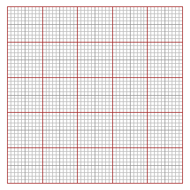 |
# In a new window, I can build a check paper (m columns, n rows) with SQUARES(m,n)
BF=4.5; HF=1.5; SQUARES(15,5)
 # With BF=3; HF=3; SQUARES(10,10) I have 10×10 squares with side 5 mm long.
#
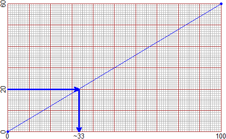
# If you have enlarged the graphic window (for example with BF=6; HF=4), with
# RATIO(tot1, tot2) you can represent the proportional transformation of data that
# connects tot1 and tot2. Start with the command INPUT(datum) or OUTPUT(datum). If you
# then use rATIO you can represent other data in the same window.
INPUT=20; RATIO(60,12)
# I obtain the left figure.
INPUT=50; RATIO(100,60)
INPUT=80; rATIO(100,60); OUTPUT=20; rATIO(100,60)
# I obtain the right figure.
# With BF=3; HF=3; SQUARES(10,10) I have 10×10 squares with side 5 mm long.
#
# If you have enlarged the graphic window (for example with BF=6; HF=4), with
# RATIO(tot1, tot2) you can represent the proportional transformation of data that
# connects tot1 and tot2. Start with the command INPUT(datum) or OUTPUT(datum). If you
# then use rATIO you can represent other data in the same window.
INPUT=20; RATIO(60,12)
# I obtain the left figure.
INPUT=50; RATIO(100,60)
INPUT=80; rATIO(100,60); OUTPUT=20; rATIO(100,60)
# I obtain the right figure.
 # Width RATIO(100,tot) or RATIO(tot,100) I can obtain the graphic representation of
# percentages. It is a convenient instrument to proportionally transform data.
# It may be subsequent to the use of graph paper:
# Width RATIO(100,tot) or RATIO(tot,100) I can obtain the graphic representation of
# percentages. It is a convenient instrument to proportionally transform data.
# It may be subsequent to the use of graph paper:
 Command INDEX
Introduction
> source("http://macosa.dima.unige.it/r.R")
Use as calculator
* / ; .
round sqrt rad2
rad3 fraction …e…
div divisors
Other calculi
= c(…) sort
[ ] min max
length sum
Figures
PLANE BF HF circle
POINT Point circle3p center3p
radius3p Colors segm
halfline line2p line
point_point inclination angle
mid2p perp2p polyline
leng […:…] polyC
Graphs
Plane abovex abovey
function graph solution
Statistics
Bar Pie Strip
distribution min max
length stem histogram
noClass median mean
Histogram morestat
More
clock GCD primes
LCM Pie(0) gonio(0)
GONIO(0) Strip(0) mmpaper1/2/3
SQUARES INPUT OUTPUT
r/RATIO
In Example of use you can find other commands. For other ones see Other examples.
Command INDEX
Introduction
> source("http://macosa.dima.unige.it/r.R")
Use as calculator
* / ; .
round sqrt rad2
rad3 fraction …e…
div divisors
Other calculi
= c(…) sort
[ ] min max
length sum
Figures
PLANE BF HF circle
POINT Point circle3p center3p
radius3p Colors segm
halfline line2p line
point_point inclination angle
mid2p perp2p polyline
leng […:…] polyC
Graphs
Plane abovex abovey
function graph solution
Statistics
Bar Pie Strip
distribution min max
length stem histogram
noClass median mean
Histogram morestat
More
clock GCD primes
LCM Pie(0) gonio(0)
GONIO(0) Strip(0) mmpaper1/2/3
SQUARES INPUT OUTPUT
r/RATIO
In Example of use you can find other commands. For other ones see Other examples.


