---------- ---------- ---------- ---------- ---------- ---------- ---------- ----------
R. 3. Other examples of use (more)
Click → here to see "Examples of use" this is an extension of.
From A to P there are developments of the parts that bear the same name. Click the
letter to see them.
From S01 to S20 there are new parts.
Click here to see an index of this paper, here for one on its own page, here for
an index of subjects.
USE as CALCULATOR
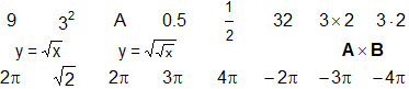
# A-B You must first write to R (only once):
source("http://macosa.dima.unige.it/r.R")
# source executes the commands that are stored in the indicated external file. We can
# use source to load commands, exercises, … from files in my computer or on Internet.
# See here for an example. See s18 for another one. Here for an example of "worksheet".
# If you expect to be unable to use the network, you can save a copy of
# http://macosa.dima.unige.it/r.R on your computer and then use "source" from the
# menu "file" to load it.
# C Other functions:
abs(3); abs(-2); sign(37); sign(-2.3); sign(0); rad4(16) rad5(-1/10^5)
# 3 2 1 -1 0 2 -0.1
# [ Although (-8)^(1/3) is -2, software calculates x^(1/3) only when x ≥ 0; so
# rad3(x) is defined as sign(x)*abs(x)^(1/3), and rad5(x) as sign(x)*abs(x)^(1/5)
# For the calculation of derivatives, use sqrt(k^2) instead of abs(k) ]
# INI_N(x) calculates the initial decimal place of the number x
INI_N(0.25); INI_N(37*1000); INI_N(-57/10000000)
# 2 3 5
# If I divide M by N, M%/%N is the integer quotient, M%%N is the remainder
750 %% 360; 750 %/% 360
# 30 2
factorial(4); choose(10,3) # factorial, binomial coeff. (see combn)
# 24 (= 4*3*2*1) 120 (= 10/3*9/2*8/1)
factorial(170); factorial(171);
# 7.257416e+306 Inf
# 171! is too large. If you type .Machine you have that 1.797693e+308 is the maximum
# usable number.
# To get a help for other functions, type: (see here)
?Math
# Other π (pi) another mathematical constant identified with a specific name, e, is the
# Napier's constant; the function exp(x) is equivalente to e^x
e; exp(1); more(e) # see "more", down
# 2.718282 2.718282 2.71828182845905
# Besides round:
trunc(2.6); floor(2.6) # truncate (to integer) instead of round
# 2 2
trunc(-7.4); floor(-7.4) # with differences on negative numbers (see)
# -7 -8
Trunc(26.47,1); Floor(26.47,1) # these also truncate to non-integers
# 26.4 26.4
Trunc(-26.47,-1); Floor(-26.47,-1)
# -20 -30
print(20/3, 2); print(20/3, 15) # round to 2, 15 digits; see "more", down.
# 6.7 6.66666666666667
signif(20/3, 2); signif(20/3, 7) # round to 2, 7 digits (7 significant digits at most)
# 6.7 6.666667
# more visualizes 15 digits, last() is the value of the last calculation
(5/13+1/7)/17; fraction(last()); more((5/13+1/7)/17)
# 0.0310278 48/1547 0.0310277957336781
# [ if A is an integer of N digits more(A) displays A correctly even if it has 16
# digits; if A has 17 digits more(A) displays all the digits but the last one can
# be wrong: a=12345678901234567; more(a) gives 12345678901234568 Why? see here]
# Some uses of circular functions
180*degrees; 180*degrees/pi; sin(30*degrees); cos(30*degrees); tan(45*degrees)
# 3.141593 1 0.5 0.8660254 1
cos(30*degrees); fraction(cos(30*degrees)/sqrt(3))
# 0.8660254 1/2 (I understand that cos(30�) = √3/2)
# I can also use WolframAlpha by introducing 0.8660254 or cos(30�) or cos(30*degrees);
# I obtain √3/2 ( "degrees" is defined so: degrees = pi/180 )
# asin, from [-1,1] to [-π/2,π/2], acos, from [-1,1] to [0,π], atan, from (-∞,∞) to
# (-π/2,π/2), are the inverse functions; for the output in degrees add "/degrees".
# D-E2 str compactly display the internal structure of an R object. Example:
str( divisors(123456) )
# num [1:28] 1 2 3 4 6 8 12 16 24 32 ... (they are 28: 1 2 3 4 6 ...)
str(sin); str(choose)
# function (x) function (n,k) (a function of 1 variable, a function of 2 variables)
# How to print a table of data. Various methods.
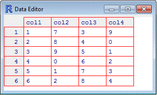
z = c(1,2,3,4,5,6,7,8,9,0,1,2,3,4,5,6,7,8,9,0,1,2,3,4); length(z)
# 24 (the data are 24; I put then in 8 columns, separated by ", "
write(z, file="",sep=', ',ncolumns=8)
# 1, 2, 3, 4, 5, 6, 7, 8
# 9, 0, 1, 2, 3, 4, 5, 6
# 7, 8, 9, 0, 1, 2, 3, 4
write(z, file="",sep='\t',ncolumns=8) # I separe the data by tabs
# 1 2 3 4 5 6 7 8
# 9 0 1 2 3 4 5 6
# 7 8 9 0 1 2 3 4
# [ I can "write" data to file; in these cases I must put file=""; if I want to write
# to the file "XX.txt" in the working directory I use: write(z, file="XX.txt", … )
# otherwise I can specify the path: write(z, file="…/XX.txt", … ) ]
# cat, that concatenates data output (and with '\n' put them in new lines), produces:
cat('',z[1:12],'\n',z[13:24],'\n')
# 1 2 3 4 5 6 7 8 9 0 1 2
# 3 4 5 6 7 8 9 0 1 2 3 4
# ( \n cab be used also with "type" and other writing commands )
# If the data have different precisions, the tabs may give rise to bad effects:
cat(20/3, 72, 15/4,'\n', 3, 1/9, 7,'\n')
# 6.666667 72 3.75
# 3 0.1111111 7
# I can make up width a tab and a rounding:
k = function(x) round(x,3)
cat('',k(20/3),'\t',k(72),'\t',k(15/4),'\n',k(3),'\t',k(1/9),'\t',k(7),'\n')
# 6.667 72 3.75
# 3 0.111 7
# or using \b to introduce a "backspace":
cat('',k(20/3),'\t\b',k(72),'\t\b\b',k(15/4),'\n',k(3),'\t\b',k(1/9),'\t\b\b',k(7),'\n')
# 6.667 72 3.75
# 3 0.111 7
# or in this way:
k = function(x) signif(x,3)
cat('',k(20/3),'\t',k(72),'\t',k(15/4),'\n',k(3),'\t',k(1/9),'\t',k(7),'\n')
# 6.67 72 3.75
# 3 0.111 7
# or opportunely by more tabs:
cat('',20/3,'\t',72,'\t\t',15/4,'\n',3,'\t\t',1/9,'\t',7,'\n')
# 6.666667 72 3.75
# 3 0.1111111 7
# cat is also convenient for printing tables. Let's see, for example, how I can print
# some binomial coefficients (we use sep="" otherwise " " is used as a separator):
# [ for(var in seq) expr repeats "expr" for all the values of "var" listed in "seq" ]
n = 5; for(k in 0:n) cat("C(", n, ",", k, ") = ", choose(n,k), sep="", '\n')
# C(5,0) = 1
# C(5,1) = 5
# C(5,2) = 10
# C(5,3) = 10
# C(5,4) = 5
# C(5,5) = 1
# See here for Pascal's triangle
# How to use cat to write (the beginning of) an irrational number ...
N=function(m) {cat("0."); for(i in 0:m) {for(j in 1:2^i) cat("0"); cat("1")}; cat("\n") }
N(0); N(1); N(2); N(5)
# 0.01
# 0.01001
# 0.0100100001
# 0.010010000100000000100000000000000001000000000000000000000000000000001
# CAT(X,N) print the sequence X of numbers or strings in rows of N columns
a=c(123,54321,356,123456,654321,13579,246810,"End"); CAT(a,4)
# 123 54321 356 123456
# 654321 13579 246810 End
x=NULL; N=4; for(i in 1:N) for(j in 1:N) x=c(x,i*j); CAT(x,N)
# 1 2 3 4
# 2 4 6 8
# 3 6 9 12
# 4 8 12 16
# Cat(x,N) produces a string that begins with the string x and ends with a sequence of
# " " so to get one of at least N characters [Cat("be",3) -> "be "; Cat("be",0) -> "be"].
m=17; n=8; p=0
cat(sep="",Cat("Mario Bianchi",m),Cat("Genova",n),Cat("via Napoli, 7",p), "\n",
Cat("Veronica Rossi",m), Cat("Milano",n),Cat("via Roma, 21",p), "\n",
Cat("Luisa Neri",m), Cat("Roma",n), Cat("via Genova, 13",p),"\n" )
# Mario Bianchi Genova via Napoli, 7
# Veronica Rossi Milano via Roma, 21
# Luisa Neri Roma via Genova, 13
#( 1234567890123456712345678 m=17; n=8)
# caT(x,N) produces a string that begins with a sequence of " " and ends with the
# string x so to get one of at least N characters.
m=14; n=9; p=17
cat(sep="",caT("Mario Bianchi",m),caT("Genova",n),caT("via Napoli, 7",p), "\n",
caT("Veronica Rossi",m), caT("Milano",n),caT("via Roma, 21",p), "\n",
caT("Luisa Neri",m), caT("Roma",n), caT("via Genova, 13",p),"\n" )
# Mario Bianchi Genova via Napoli, 7
# Veronica Rossi Milano via Roma, 21
# Luisa Neri Roma via Genova, 13
#( 1234567890123412345678912345678901234567 m=14; n=9; p=17)
Other CALCULI
# F-G1 I can use an indexed variable (or vector), for example I can write XX[3]=8,
# only if I have already used XX. A simplwe way is to make this assignment: XX = NULL.
# Example:
for(i in 1:9) W[i] = i*2; W # If I have never used W:
# Error in W[i] = i * 2 : object "W" not found
W = NULL; for(i in 1:9) W[i] = i*2; W
# [1] 2 4 6 8 10 12 14 16 18
# A more general way is to define the length of the vector XX:
Z = vector( length=9) ; for(i in 1:9) Z[i] = i*2; Z
# [1] 2 4 6 8 10 12 14 16 18
# prod (like sum) returns the product of all the values present in its arguments:
x = c(2, 3, 7, 100); prod(x)
# 4200
# reverse returns the arguments in reverse order
x = c(2, 3, 7, 100); y = reverse(x); y
# [1] 100 7 3 2
# combn(x,N) generate all combinations of the elements of x taken N at a time
x = c(2, 3, 7, 100); combn(x,2)
# [,1] [,2] [,3] [,4] [,5] [,6]
# [1,] 2 2 2 3 3 7
# [2,] 3 7 100 7 100 100 They are 6 = choose(4,2) (see)
combn(x,3)
# [,1] [,2] [,3] [,4]
# [1,] 2 2 2 3
# [2,] 3 3 7 7
# [3,] 7 100 100 100 They are 4 = choose(4,3)
# Interval computation. + - * / ^:
# The area of the rectangle with one side between 30.5 and 31.5 and the other between
# 1.3 and 1.4 cm [put as operand a certain number or the pair of extremes of the
# interval in which it is]:
approx( c(30.5, 31.5), c(1.3, 1.4), "*")
# [1] min 39.65 [2] max 44.10
approx2( c(30.5, 31.5), c(1.3, 1.4), "*")
# [1] center 41.875 [2] radius 2.225
# It is in [39.65 cm², 44.10 cm²], or: 41.9 ± 2.3 cm²
# The double of the first side:
approx( c(30.5, 31.5), 2, "*")
# [1] min 61 [2] max 63 it is 62 ± 1 cm
# Idem for +, -, /, ^.
# Another example:
x = 2.1 ± 0.1, y = 2.9 ± 0.1, 1/z = 1/x + 1/y. How much is z?
x = c(2.0, 2.2); y = c(2.8, 3.0)
rx = approx(1,x, "/"); rx # 0.4545455 0.5000000
ry = approx(1,y, "/"); ry # 0.3333333 0.3571429
rz = approx(rx,ry, "+"); rz # 0.7878788 0.8571429
z = approx(1,rz, "/"); z
# [1] min 1.166667 [2] max 1.269231
# or:
approx2(1,rz, "/")
# [1] center 1.21794872 [2] radius 0.05128205
# or alternatively: 1.22 ± 0.06
# Other example (see here):
 # catheti: 22 ≤ a ≤ 23, 38 ≤ b ≤ 39 → hypotenuse: 43.9 ≤ c ≤ 45.3
# In other situations (if there are other functions or a variable appears more than
# once) I can use EPS(r) that generates random values from -r to r. An example.
# A marble is launched in the air with initial speed v=4±0.1 m/s. After t=0.6±0.06 s
# it reaches the height h = v*t-g*t^2/2, where g = 9.80±0.001 m/s^2. How tall is h?
t = 0.6+EPS(0.06); v = 4+EPS(0.1); g = 9.8+EPS(0.001)
h = function(t,v,g) v*t-g*t^2/2; m=min( h(t,v,g) ); M=max( h(t,v,g) ); m; M
# 0.4394657 0.7852536 h is between these value, or:
(m+M)/2; (M-m)/2
# 0.6123597 0.1728939 h = 0.612 +/- 0.173, or h = 0.6 +/- 0.2 (m)
# (the solutions with more figures do not make sense!)
FIGURES
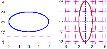
# H-I If I put ASP = k before PLANE (monometric plane) I can change the aspect ratio
# between the units of y-axis and x-axis. If I move the window ASP doesn't change.
BF=2.6; HF=2.6
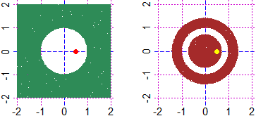
ASP = 1/2; PLANE(-2,2, -4,4); circle(0,0, 2, "blue")
ASP = 3; PLANE(-6,6, -2,2); circle(0,0, 2, "brown")
# catheti: 22 ≤ a ≤ 23, 38 ≤ b ≤ 39 → hypotenuse: 43.9 ≤ c ≤ 45.3
# In other situations (if there are other functions or a variable appears more than
# once) I can use EPS(r) that generates random values from -r to r. An example.
# A marble is launched in the air with initial speed v=4±0.1 m/s. After t=0.6±0.06 s
# it reaches the height h = v*t-g*t^2/2, where g = 9.80±0.001 m/s^2. How tall is h?
t = 0.6+EPS(0.06); v = 4+EPS(0.1); g = 9.8+EPS(0.001)
h = function(t,v,g) v*t-g*t^2/2; m=min( h(t,v,g) ); M=max( h(t,v,g) ); m; M
# 0.4394657 0.7852536 h is between these value, or:
(m+M)/2; (M-m)/2
# 0.6123597 0.1728939 h = 0.612 +/- 0.173, or h = 0.6 +/- 0.2 (m)
# (the solutions with more figures do not make sense!)
FIGURES
# H-I If I put ASP = k before PLANE (monometric plane) I can change the aspect ratio
# between the units of y-axis and x-axis. If I move the window ASP doesn't change.
BF=2.6; HF=2.6
ASP = 1/2; PLANE(-2,2, -4,4); circle(0,0, 2, "blue")
ASP = 3; PLANE(-6,6, -2,2); circle(0,0, 2, "brown")
 # You can save the current plot and to replay it (after you've opened a new graphics
# device). If I type Name = recordPlot() (Name is any name) the plot is saved; if I
# open a new grapics window later and type replayPlot(Name) the old object reappears
# and I can work it again [if you want delete the latest device you can use dev.off();
# dev.new() open a new device; the two commands can be useful to realize animations; I
# use dev.new(width=b,height=h) - or dev.new(width=BF,height=HF) - if I want a device
# like that obtained with BF=b; HF=h].
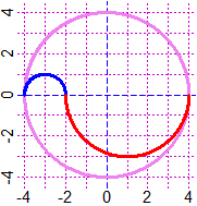
# With ARC(xCenter,yCenter, radius, from,to, col) I draw arcs of a circle:
HF=2.5; BF=2.5; PLANE(-4,4, -4,4); circle(0,0, 4, "violet")
ARC(-3,0, 1, 0,180, "blue"); ARC(1,0, 3, 180,360, "red")
# You can save the current plot and to replay it (after you've opened a new graphics
# device). If I type Name = recordPlot() (Name is any name) the plot is saved; if I
# open a new grapics window later and type replayPlot(Name) the old object reappears
# and I can work it again [if you want delete the latest device you can use dev.off();
# dev.new() open a new device; the two commands can be useful to realize animations; I
# use dev.new(width=b,height=h) - or dev.new(width=BF,height=HF) - if I want a device
# like that obtained with BF=b; HF=h].
# With ARC(xCenter,yCenter, radius, from,to, col) I draw arcs of a circle:
HF=2.5; BF=2.5; PLANE(-4,4, -4,4); circle(0,0, 4, "violet")
ARC(-3,0, 1, 0,180, "blue"); ARC(1,0, 3, 180,360, "red")
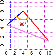
 # Another example (a right-angle triangle):
PLANE(-1,10, -1,10)
segm(9,1, 3,8, "red"); inclination(9,1, 3,8)
# [1] -49.39871 (inclination of red segment)
# I draw a 5 long segment form 3,8 towards the direction by 90� decreased
Direction(3,8, inclination(9,1, 3,8)-90, 5, "blue")
# I draw a segment from the arrival point to 9,1
segm(Directionx,Directiony, 9,1, "violet")
# I draw the arc (with center 3,8 and radius 2) that goes from side to side
ARC(3,8, 2, inclination(9,1, 3,8)-90, inclination(9,1, 3,8), "orange")
type(3,5,"90�")
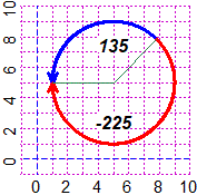
# The third figure uses the command ARCd, which draws an arrow to give a direction
# to the arc.
PLANE(-1,10, -1,10)
ARCd(5,5, 4, 45,180, "blue"); ARCd(5,5, 4, 45,-180, "red")
Directio(5,5, 180,4, "seagreen"); Directio(5,5, 45,4, "seagreen")
CLEAN(4,6, 7,8); text(5,7.5, "135",font=4)
CLEAN(4,6, 2,3); text(5,2.5,"-225",font=4)
# circl and circl2, circl3p arc arcd draw thinner lines than circle, circle3p, ARC, ARCd.
# halfl, l2p and p2p draw thinner lines than halfline, line2p and perp2p.
# polylin and polyl draw thinner or much thinner lines than polyline; polyli makes use
# of dashed lines.
# Another example (a right-angle triangle):
PLANE(-1,10, -1,10)
segm(9,1, 3,8, "red"); inclination(9,1, 3,8)
# [1] -49.39871 (inclination of red segment)
# I draw a 5 long segment form 3,8 towards the direction by 90� decreased
Direction(3,8, inclination(9,1, 3,8)-90, 5, "blue")
# I draw a segment from the arrival point to 9,1
segm(Directionx,Directiony, 9,1, "violet")
# I draw the arc (with center 3,8 and radius 2) that goes from side to side
ARC(3,8, 2, inclination(9,1, 3,8)-90, inclination(9,1, 3,8), "orange")
type(3,5,"90�")
# The third figure uses the command ARCd, which draws an arrow to give a direction
# to the arc.
PLANE(-1,10, -1,10)
ARCd(5,5, 4, 45,180, "blue"); ARCd(5,5, 4, 45,-180, "red")
Directio(5,5, 180,4, "seagreen"); Directio(5,5, 45,4, "seagreen")
CLEAN(4,6, 7,8); text(5,7.5, "135",font=4)
CLEAN(4,6, 2,3); text(5,2.5,"-225",font=4)
# circl and circl2, circl3p arc arcd draw thinner lines than circle, circle3p, ARC, ARCd.
# halfl, l2p and p2p draw thinner lines than halfline, line2p and perp2p.
# polylin and polyl draw thinner or much thinner lines than polyline; polyli makes use
# of dashed lines.
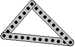 |
See here how to make this image of a building made with the Meccano. |
# arcC(a,b,R, u,v,C) draws the circular sector (with center a,b and radius R) from u�
# to v� in color C
PLANEww(-5,5,-5,5); B="brown"
arcC(0,0,5, -30,50,"green"); arcC(0,0,5, 50,130,"blue")
arcC(0,0,5, 130,210,"yellow")
ARC(0,0,5, -30,210, B)
Direction(0,0,-30,5,B); Direction(0,0,50,5,B)
Direction(0,0,130,5,B); Direction(0,0,210,5,B) |
 |
# "Black" can be specified by 1. Other colors can be specified by giving an index.
# With Ncolor() I can quote the numbers associated with these colors:
Ncolor()
#1 black, 2 red, 3 green, 4 blue, 5 cyan, 6 violet, 7 yellow, 8 grey
# (then: 9 is black, 10 is red, ...)
HF=1; BF=4; PLANE(0,21,-1,1); for (c in 1:20) POINT(c,0, c)
 # Alternatively, colors can be specified directly with a string of the form rgb(a,b,c)
# where each of numbers a,b,c has a value in the range 0 to 1 that states the quantity
# of red,green,blue: POINT(2,3, rgb(1,0,0) ) draw (2,3) red, POINT(4,5, rgb(1,0.5,0) )
# draw (4,5) orange, POINT(3,2, rgb(0.7,0.7,0.7) ) draw (3,2) grey.
# I can also use colors() to get more names than those obtainable with Colors().
# Other pictures here
# Alternatively, colors can be specified directly with a string of the form rgb(a,b,c)
# where each of numbers a,b,c has a value in the range 0 to 1 that states the quantity
# of red,green,blue: POINT(2,3, rgb(1,0,0) ) draw (2,3) red, POINT(4,5, rgb(1,0.5,0) )
# draw (4,5) orange, POINT(3,2, rgb(0.7,0.7,0.7) ) draw (3,2) grey.
# I can also use colors() to get more names than those obtainable with Colors().
# Other pictures here
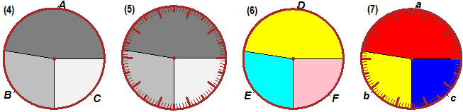
 # J-J6 If I type Quadrilateral(a,b,c,d) width 4 directions (numbers ranging from 0
# to 360) instead of a,b,c,d I obtain:
# J-J6 If I type Quadrilateral(a,b,c,d) width 4 directions (numbers ranging from 0
# to 360) instead of a,b,c,d I obtain:
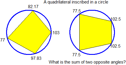 # [ the first figure has been obtained with Quadrilateral(0,80,195.67,286) ]
# You can easily build similar "problems".
# P() allows you to click on a point and read its coordinates. Example:
HF=3; BF=3; PLANE(0,10, 0,10)
P() # I click (more or less) the point 5,9 and I obtain
# xP = 4.989773 ; yP = 9.005114 or something like that
# See here.
# PPP() store the coordinates of the clicked point by the names xP and yP
# (we have seen here how it can be usefully employed in the basic school)
# NW() prepares a new window of the same dimensions as the last one.
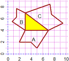
# polyS, polyS2 act like polyC but they emphasize the polygon by shading lines (± dense)
# with a given angle (rather than with a color); see the left figure.
BF=3;HF=3; PLANE(-1,5, -1,5)
x = c(-1,1,5,2); y = c(0,-1,2,4); polyS(x,y, 45, "red")
x1 = c(0,3,5); y1 = c(5,-1,1); polyS2(x1,y1, -45, "seagreen")
# [ the first figure has been obtained with Quadrilateral(0,80,195.67,286) ]
# You can easily build similar "problems".
# P() allows you to click on a point and read its coordinates. Example:
HF=3; BF=3; PLANE(0,10, 0,10)
P() # I click (more or less) the point 5,9 and I obtain
# xP = 4.989773 ; yP = 9.005114 or something like that
# See here.
# PPP() store the coordinates of the clicked point by the names xP and yP
# (we have seen here how it can be usefully employed in the basic school)
# NW() prepares a new window of the same dimensions as the last one.
# polyS, polyS2 act like polyC but they emphasize the polygon by shading lines (± dense)
# with a given angle (rather than with a color); see the left figure.
BF=3;HF=3; PLANE(-1,5, -1,5)
x = c(-1,1,5,2); y = c(0,-1,2,4); polyS(x,y, 45, "red")
x1 = c(0,3,5); y1 = c(5,-1,1); polyS2(x1,y1, -45, "seagreen")
 # See here for the construction of the center and left figures, and for the use of the
# commands: polySN(x,y, angle, N, col) for other shading lines,
# text(x,y,text, font=N) and the options to change alignment, size, color, font, string,
# rotation, family,
# dart2, arrow2, Dart2, Arrow2 that connect the top of the preceding arrow with the top
# of the new one. With arroW2 and ArroW2 I have an intermediate thickness between
# "dart" and "arrow".
# See here for the construction of the center and left figures, and for the use of the
# commands: polySN(x,y, angle, N, col) for other shading lines,
# text(x,y,text, font=N) and the options to change alignment, size, color, font, string,
# rotation, family,
# dart2, arrow2, Dart2, Arrow2 that connect the top of the preceding arrow with the top
# of the new one. With arroW2 and ArroW2 I have an intermediate thickness between
# "dart" and "arrow".# Some examples of writing (on a coloured background):
PLANE(0,6, 0,6)
x=c(1,6,6,1); y=c(1,1,6,6); polyC(x,y, "grey")
type(2,2,"A\nB"); typeC(3,2,"grey","C\nD")
typeC(4,2, 0,"E\nF"); typeR(2,4, 30,"G\nH")
typeRC(3,4, 30, 0,"I\nL"); text(4.5,5, font=4,srt=45,"M\nN")
text(5.3,2.5, font=4, cex=1.2, srt=180,"O\nP")
# If you want superimpose any white rectangle before writing see S18 | 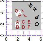 |
# With type and text, I can use bquote(2*pi) and bquote(sqrt(3)) to obtain 2π and √3.
# For other formulas that I can obtain with bquote, see here. Examples:
# A lot of geometrical problems can be easily solved.
See here for an example. | 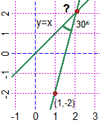 |
# Direction(x,y, d,r, col) with the color 0 doesn't draw the "radius", but in Directionx
# and Directiony there are the coordinates of the arrival point. An example: (see here)
 # Here are some other commands that are useful for drawing figures.
# I can shift with a translation, rotate and multiply the points by:
# MulTraRot(x,y, mx,my, tx,ty, ang) and RotTraMul(x,y, ang, tx,ty, mx,my). The
# first multiply the coordinates by mx and my, then shift by tx,ty and finally rotates
# the point about (0,0) by ang�. The second produces first a rotation about (0,0),
# then a translation and finally a multiplication of the coordinates. If I add [1] or
# [2] to the command I have the 1st or the 2nd coordinate. To operate on curves see S01.
# We have seen here symm(x,y, A,B, C,D) and symm2(x,y, A,B, d) to obtain the symmetric
# of x,y with respect to the line through (A,B) and (C,D) or through (A,B) with the
# direction of d degrees.
# RotP(x,y, ang, x0,y0) rotates (x,y) about (x0,y0) by ang�.
# RotPx(x,y, ang, x0,y0), RotPy(x,y, ang, x0,y0) give his two coordinates.
# MulRotP(x,y, m, ang, x0,y0) multiply by m the distance of (x,y) from (x0,y0) and
# rotates it about (x0,y0) by ang�.
# See here for an example, that generates the following immage.
# Here are some other commands that are useful for drawing figures.
# I can shift with a translation, rotate and multiply the points by:
# MulTraRot(x,y, mx,my, tx,ty, ang) and RotTraMul(x,y, ang, tx,ty, mx,my). The
# first multiply the coordinates by mx and my, then shift by tx,ty and finally rotates
# the point about (0,0) by ang�. The second produces first a rotation about (0,0),
# then a translation and finally a multiplication of the coordinates. If I add [1] or
# [2] to the command I have the 1st or the 2nd coordinate. To operate on curves see S01.
# We have seen here symm(x,y, A,B, C,D) and symm2(x,y, A,B, d) to obtain the symmetric
# of x,y with respect to the line through (A,B) and (C,D) or through (A,B) with the
# direction of d degrees.
# RotP(x,y, ang, x0,y0) rotates (x,y) about (x0,y0) by ang�.
# RotPx(x,y, ang, x0,y0), RotPy(x,y, ang, x0,y0) give his two coordinates.
# MulRotP(x,y, m, ang, x0,y0) multiply by m the distance of (x,y) from (x0,y0) and
# rotates it about (x0,y0) by ang�.
# See here for an example, that generates the following immage.
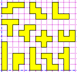 # The immage on the right recalls some activities with the pentominoes described here.
# After drawing a line or an arrow (with segm, line, arrow, dash, ...), the end point
# coordinates are stored in xend and yend. This can be useful for building various
# types of figures. An initial point can be traced with Dot: its coordinates are put
# in xend, yend. See here for an example, that produce the figure above, on the right.
# Dot2 traced a point large 3 pixel.
GRAPHS
# K Other ways of putting inscriptions along the axes
# On the left:
year = c(1880,1890,1900,1910,1920,1930,1940,1950,1960,1970,1980)
fruit = c(19, 21, 23, 28, 31, 27, 23, 37, 65, 88, 79)
BF=4; HF=2.5
Grid(1880,1980, 0,90)
polyline(year,fruit, "blue"); POINT(year,fruit, "brown")
underx("year"); underX(1880,1880); underX(1980,1980)
# underx(n) writes the name n in the center, underX(n, p) in the position p
undery("fruit"); aboveY(90,90); aboveY(0,0); aboveY(50,50)
# The immage on the right recalls some activities with the pentominoes described here.
# After drawing a line or an arrow (with segm, line, arrow, dash, ...), the end point
# coordinates are stored in xend and yend. This can be useful for building various
# types of figures. An initial point can be traced with Dot: its coordinates are put
# in xend, yend. See here for an example, that produce the figure above, on the right.
# Dot2 traced a point large 3 pixel.
GRAPHS
# K Other ways of putting inscriptions along the axes
# On the left:
year = c(1880,1890,1900,1910,1920,1930,1940,1950,1960,1970,1980)
fruit = c(19, 21, 23, 28, 31, 27, 23, 37, 65, 88, 79)
BF=4; HF=2.5
Grid(1880,1980, 0,90)
polyline(year,fruit, "blue"); POINT(year,fruit, "brown")
underx("year"); underX(1880,1880); underX(1980,1980)
# underx(n) writes the name n in the center, underX(n, p) in the position p
undery("fruit"); aboveY(90,90); aboveY(0,0); aboveY(50,50)
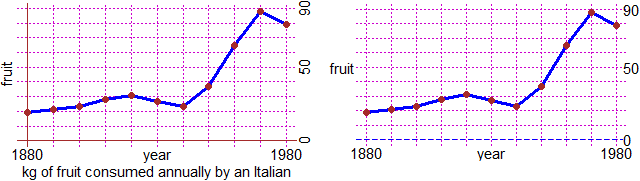 # With AXES(a,b,"Col") I can trace two axes of color Col through (a,b). In the picture:
AXES(1880,0,"brown")
# AXES2 tracks them thicker. underx2 writes in the line below.
underx2("kg of fruit consumed annually by an Italian")
# On the right:
# ...
UnderY("fruit",50); AboveY(90,90); AboveY(0,0); AboveY(50,50)
# or: n=c(0,50,90); for(i in 1:3) AboveY(n[i],n[i])
# Other commands are underY, aboveX, AboveX, UnderX (in addition to abovex, abovey).
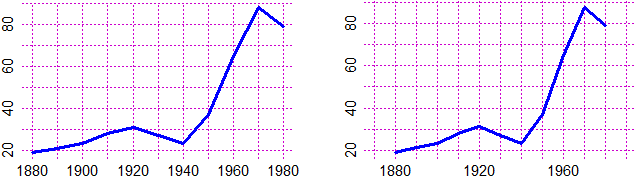
# If in x and y there are the coordinates of some points, PlaneP(x,y) automatically
# chooses a "plane" that contains all of them (it is simliar to graphF for functions);
# PLANEP(x,y) chooses it monometric. For the sake of brevity we use the preceding data:
PlaneP(year,fruit); polyline(year,fruit, "blue")
PLANEP(year,fruit); polyline(year,fruit, "blue")
# With AXES(a,b,"Col") I can trace two axes of color Col through (a,b). In the picture:
AXES(1880,0,"brown")
# AXES2 tracks them thicker. underx2 writes in the line below.
underx2("kg of fruit consumed annually by an Italian")
# On the right:
# ...
UnderY("fruit",50); AboveY(90,90); AboveY(0,0); AboveY(50,50)
# or: n=c(0,50,90); for(i in 1:3) AboveY(n[i],n[i])
# Other commands are underY, aboveX, AboveX, UnderX (in addition to abovex, abovey).
# If in x and y there are the coordinates of some points, PlaneP(x,y) automatically
# chooses a "plane" that contains all of them (it is simliar to graphF for functions);
# PLANEP(x,y) chooses it monometric. For the sake of brevity we use the preceding data:
PlaneP(year,fruit); polyline(year,fruit, "blue")
PLANEP(year,fruit); polyline(year,fruit, "blue")
 # range (see) gives min/max of some data, RANGE estimate min/max of a function between
# 2 input (if the function had a bump we could use maxmin - see):
range(fruit)
#19 88
f = function(x) (x+1/3)^2+1; RANGE(f, -5,10)
#"~ min F(min) Max F(Max) mfMf[1:4] = "
# -0.3333303 1.0000000 10.0000000 107.7777778
RANGE(f,-0.5,0)
#"~ min F(min) Max F(Max) mfMf[1:4] = "
# -0.3333333 1.0000000 0.0000000 1.1111111
mfMf[1]; mfMf[2]
# -0.3333333 1.0000000
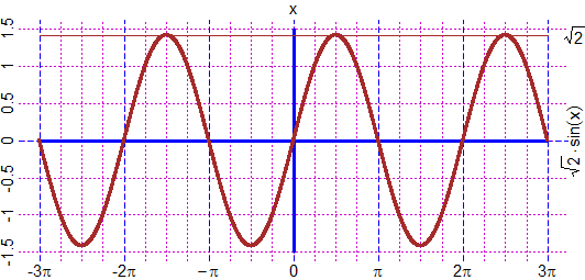
RANGE(sin, -5,10)
#"~ min F(min) Max F(Max) mfMf[1:4] = "
# 4.71239 -1.00000 -4.71239 1.00000
Two of the various min/max __/
# range (see) gives min/max of some data, RANGE estimate min/max of a function between
# 2 input (if the function had a bump we could use maxmin - see):
range(fruit)
#19 88
f = function(x) (x+1/3)^2+1; RANGE(f, -5,10)
#"~ min F(min) Max F(Max) mfMf[1:4] = "
# -0.3333303 1.0000000 10.0000000 107.7777778
RANGE(f,-0.5,0)
#"~ min F(min) Max F(Max) mfMf[1:4] = "
# -0.3333333 1.0000000 0.0000000 1.1111111
mfMf[1]; mfMf[2]
# -0.3333333 1.0000000
RANGE(sin, -5,10)
#"~ min F(min) Max F(Max) mfMf[1:4] = "
# 4.71239 -1.00000 -4.71239 1.00000
Two of the various min/max __/ 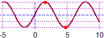 # RANGE0 is less precise but faster than RANGE
RANGE0(f, -0.5,10)
#"~ min F(min) Max F(Max) mfMf[1:4] = "
# -0.3330333 1.0000001 10.0000000 107.7777778
#
# Using these commands I can easily get any type of chart; it can be useful for teachers:
# two examples referring to typical activities of the first years of school (see):
# RANGE0 is less precise but faster than RANGE
RANGE0(f, -0.5,10)
#"~ min F(min) Max F(Max) mfMf[1:4] = "
# -0.3330333 1.0000001 10.0000000 107.7777778
#
# Using these commands I can easily get any type of chart; it can be useful for teachers:
# two examples referring to typical activities of the first years of school (see):
 # K1-K2 In addition to graphs of 1 variable functions, I can plot curves described as
# functions of 2 variables using the command CURVE(K, col). Examples:
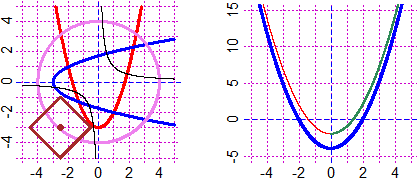
PLANE(-5,5, -5,5)
f = function(x,y) y-(x^2-3); CURVE(f, "red") # parabola
g = function(x,y) x-(y^2-3); CURVE(g, "blue") # parabola
h = function(x,y) x^2+y^2-16; CURVE(h, "violet") # circle
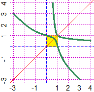
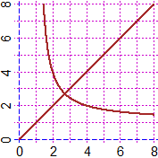
k = function(x,y) x*y-1; CUR(k, "black") # hyperbola
t = function(x,y) dist_taxi(x,y, -2.5,-3)-2
CURVE(t,"brown"); POINT(-2.5,-3, "brown")
# where dist_taxi(x1,y1,x2,y2) is the taxicab (or Manhattan) distance: |Δx|+|Δy|
# For other ways to describe curves, see here [the conics] and the S01 section.
# To solve eq. of type F(x,y) = 0 with respect to x (fixed y=k) or y (fixed x=k) see
# here
# CUR tracks thin-stroke curves; CURV uses an intermediate thickness.
# K1-K2 In addition to graphs of 1 variable functions, I can plot curves described as
# functions of 2 variables using the command CURVE(K, col). Examples:
PLANE(-5,5, -5,5)
f = function(x,y) y-(x^2-3); CURVE(f, "red") # parabola
g = function(x,y) x-(y^2-3); CURVE(g, "blue") # parabola
h = function(x,y) x^2+y^2-16; CURVE(h, "violet") # circle
k = function(x,y) x*y-1; CUR(k, "black") # hyperbola
t = function(x,y) dist_taxi(x,y, -2.5,-3)-2
CURVE(t,"brown"); POINT(-2.5,-3, "brown")
# where dist_taxi(x1,y1,x2,y2) is the taxicab (or Manhattan) distance: |Δx|+|Δy|
# For other ways to describe curves, see here [the conics] and the S01 section.
# To solve eq. of type F(x,y) = 0 with respect to x (fixed y=k) or y (fixed x=k) see
# here
# CUR tracks thin-stroke curves; CURV uses an intermediate thickness.
# An example [see:
# here]:
#
# 2^(x*y) = x+y
# ( and y = x )
|   |
# Another:
f=function(x,y) x^y - y^x
BF=2.5; HF=2.5
PLANE(0,8, 0,8)
CURV(f, "brown")
# [ when x>0, y>0;  but
#   we have also, ie:
#   (-2)^(-4) = 1/2^4 =
#   0.0625 = (-4)^(-2)  ]
# (e,e) is a double point
|  |
# An egg:
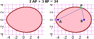 A=c(-4,0); B=c(3,0)
F = function(x,y) 2*point_point(A[1],A[2],x,y)+3*point_point(B[1],B[2],x,y)-24
BF=2.5; HF=2; PLANE(-5,5, -4,4); CURVE(F, "brown")
# How to color the interior (see here):
for(i in 1:10) Diseq1(F,0, "pink")
CURVE(F, "brown"); POINT(A[1],A[2],"blue"); POINT(B[1],B[2],"blue")
# Likewise, graph1F and graph1 work in the same way as graphF and graph but with
# thin-stroke curves. graph2F and graph2 make them with an intermediate thickness.
Plane(-5,5, -5,15)
q = function(x) x^2-4; graph(q,-5,5, "blue")
s = function(x) x^2-2; graph1(s,-5,0, "red"); graph2(s,0,5, "seagreen")
# f, g, h, k q, s
A=c(-4,0); B=c(3,0)
F = function(x,y) 2*point_point(A[1],A[2],x,y)+3*point_point(B[1],B[2],x,y)-24
BF=2.5; HF=2; PLANE(-5,5, -4,4); CURVE(F, "brown")
# How to color the interior (see here):
for(i in 1:10) Diseq1(F,0, "pink")
CURVE(F, "brown"); POINT(A[1],A[2],"blue"); POINT(B[1],B[2],"blue")
# Likewise, graph1F and graph1 work in the same way as graphF and graph but with
# thin-stroke curves. graph2F and graph2 make them with an intermediate thickness.
Plane(-5,5, -5,15)
q = function(x) x^2-4; graph(q,-5,5, "blue")
s = function(x) x^2-2; graph1(s,-5,0, "red"); graph2(s,0,5, "seagreen")
# f, g, h, k q, s
 # Not all curves have a curved shape:
F = function(x,y) sqrt(x^2+y^2)-2*sqrt(x*y); PLANE(-3,3, -3,3); CURV(F,"seagreen")
G = function(x,y) x^2*y-x*y^2+x*y*sqrt(x*y); PLANE(-3,3, -3,3); CURV(G,"brown")
# Not all curves have a curved shape:
F = function(x,y) sqrt(x^2+y^2)-2*sqrt(x*y); PLANE(-3,3, -3,3); CURV(F,"seagreen")
G = function(x,y) x^2*y-x*y^2+x*y*sqrt(x*y); PLANE(-3,3, -3,3); CURV(G,"brown")
 # NOTE. graph and graphF take enough time to plot the graphs, but they make them very
# precisely. See here to pay attention to the use of CURVE and plot (that we have not
# discussed so far). The following figure shows the graphs of some functions that have
# jumps, both those obtained with graph and those, incorrect, obtained with CURVE and
# plot.
# Here you see the use of GRAPH, GRAPH1, GRAPH2, faster than graph, graph1, graph2.
# NOTE. graph and graphF take enough time to plot the graphs, but they make them very
# precisely. See here to pay attention to the use of CURVE and plot (that we have not
# discussed so far). The following figure shows the graphs of some functions that have
# jumps, both those obtained with graph and those, incorrect, obtained with CURVE and
# plot.
# Here you see the use of GRAPH, GRAPH1, GRAPH2, faster than graph, graph1, graph2.
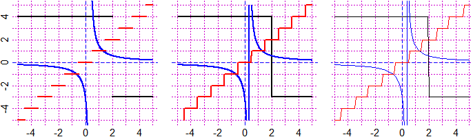 # The graph of a function does not display the possible holes: points where it is not
# defined (or where it is non continuos). Here's how to proceed in these cases.
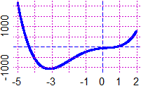
HF=2.5; BF=3; F=function(x) (x^5+x^4-3*x^2-2*x+1)/(x^4-3*x+1); graphF(F, -2,4, "brown")
# I get (A). But F is non defined where x^4-3*x+1=0. Where?
# The graph of a function does not display the possible holes: points where it is not
# defined (or where it is non continuos). Here's how to proceed in these cases.
HF=2.5; BF=3; F=function(x) (x^5+x^4-3*x^2-2*x+1)/(x^4-3*x+1); graphF(F, -2,4, "brown")
# I get (A). But F is non defined where x^4-3*x+1=0. Where?
 graphF(F, -2,4, "brown"); G = function(x) x^4-3*x+1; graph1(G,-4,6, "red")
A=solution(G,0, 0,1); B=solution(G,0, 1,1.5); A; B; POINT(c(A,B),c(0,0),"black")
# 0.3376668 1.307486
E=1e-10; POINT(A+E,F(A+E),"yellow"); POINT(B+E,F(B+E),"yellow")
# For painting the holes I drew (in yellow color) points on the graph with abscissa
# close to that of the holes. I get (B). The final graph, (C):
graph2F(F,-2,4, "brown"); pointO(A+E,F(A+E),"blue"); pointO(B+E,F(B+E),"blue")
# We have seen how to calculate the distance of a point from another one or a straight
# line. distPF(x,y, F, a,b) calculates the distance between a point x,y and the graph
# of a 1-input-1-output function F in the domain a,b.
# Let's see, for example, how to calculate the distances of (2,0) - blue point - from
# both K and G (I want to understand which of the two curves is closest to the point)
graphF(F, -2,4, "brown"); G = function(x) x^4-3*x+1; graph1(G,-4,6, "red")
A=solution(G,0, 0,1); B=solution(G,0, 1,1.5); A; B; POINT(c(A,B),c(0,0),"black")
# 0.3376668 1.307486
E=1e-10; POINT(A+E,F(A+E),"yellow"); POINT(B+E,F(B+E),"yellow")
# For painting the holes I drew (in yellow color) points on the graph with abscissa
# close to that of the holes. I get (B). The final graph, (C):
graph2F(F,-2,4, "brown"); pointO(A+E,F(A+E),"blue"); pointO(B+E,F(B+E),"blue")
# We have seen how to calculate the distance of a point from another one or a straight
# line. distPF(x,y, F, a,b) calculates the distance between a point x,y and the graph
# of a 1-input-1-output function F in the domain a,b.
# Let's see, for example, how to calculate the distances of (2,0) - blue point - from
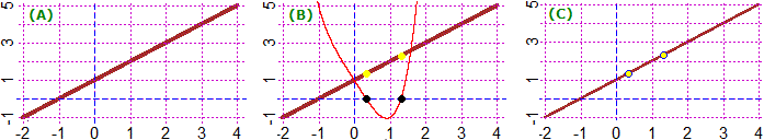
# both K and G (I want to understand which of the two curves is closest to the point)
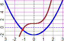
 PLANE(-1,2, -1,2)
K = function(x) 2*x-0.5; graph(K,-1,2, "red")
G = function(x) x^2; graph(G,-1,2, "brown")
POINT(2,-1, "blue"); distPF(2,-1, K, -1,2)
#dist. & nearest point (punto pi� vicino):
# 2.012461 0.200000 -0.100000
POINT(0.2,-0.1, "black"); line(0.2,-0.1, 2,-1, "blue")
# in this case I would also find the distance with the point_line command
point_line(2,-1, 0,-1/2, 1,1.5)
# 2.012461
# For G, whose chart is not a straight line, I can not do it.
distPF(2,-1, G, -1,2)
#dist. & nearest point (punto pi� vicino):
# 1.9490881 0.5535740 0.3064442
# I can improve accuracy starting from a smaller interval.
distPF(2,-1, G, 0.5,0.6)
# 1.9490881 0.5535738 0.3064440
POINT(0.5535740, 0.3064442, 1); line(0.5535740, 0.3064442, 2,-1, "blue")
# The curve G is closer
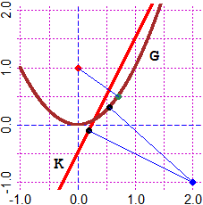
# Let us calculate the distance of the red point, (0,1), from G:
POINT(0,1, "red"); distPF(0,1, G, -1,2)
# 0.8660254 -0.7071070 0.5000003 I can improve precision:
distPF(0,1, G, -0.8,-0.6)
# 0.8660254 -0.7071068 0.5000000
# These numbers look like all square roots of fractions between integers. Check:
fraction(distPF(0,1, G, -0.8,-0.6)^2)
# 0.8660254 -0.7071068 0.5000000
# 3/4 1/2 1/4 The distance is √3/2
# I plot (0.707…, 0.5)
POINT(sqrt(1/2), 1/2, "seagreen"); line(0,1, sqrt(1/2),1/2, "blue")
# NOTE: CURVE(h,…) to build the graph of h(x,y)=0 looks where h changes the sign; if
# h(x,y)≥0 or h(x,y)≤0 everywhere, the graph is not traced. Then try to operate, as
# illustrated below, with the CURVEN (or CURN) command (see here for more information).
PLANE(-4,4, -4,4)
g = function(x,y) x^2+4*y^2-4*x*y; CURVE(g,"green")
# I get nothing ( though in this case I know the curve is
# x-2*y = 0 because x^2+4*y^2-4*x*y = (x-2*y)^2 )
CURVEN(g,1, "blue") # CURN(g,1, "brown")
#[ y = F(x) +/- 1e-04 ]
PLANE(-1,2, -1,2)
K = function(x) 2*x-0.5; graph(K,-1,2, "red")
G = function(x) x^2; graph(G,-1,2, "brown")
POINT(2,-1, "blue"); distPF(2,-1, K, -1,2)
#dist. & nearest point (punto pi� vicino):
# 2.012461 0.200000 -0.100000
POINT(0.2,-0.1, "black"); line(0.2,-0.1, 2,-1, "blue")
# in this case I would also find the distance with the point_line command
point_line(2,-1, 0,-1/2, 1,1.5)
# 2.012461
# For G, whose chart is not a straight line, I can not do it.
distPF(2,-1, G, -1,2)
#dist. & nearest point (punto pi� vicino):
# 1.9490881 0.5535740 0.3064442
# I can improve accuracy starting from a smaller interval.
distPF(2,-1, G, 0.5,0.6)
# 1.9490881 0.5535738 0.3064440
POINT(0.5535740, 0.3064442, 1); line(0.5535740, 0.3064442, 2,-1, "blue")
# The curve G is closer
# Let us calculate the distance of the red point, (0,1), from G:
POINT(0,1, "red"); distPF(0,1, G, -1,2)
# 0.8660254 -0.7071070 0.5000003 I can improve precision:
distPF(0,1, G, -0.8,-0.6)
# 0.8660254 -0.7071068 0.5000000
# These numbers look like all square roots of fractions between integers. Check:
fraction(distPF(0,1, G, -0.8,-0.6)^2)
# 0.8660254 -0.7071068 0.5000000
# 3/4 1/2 1/4 The distance is √3/2
# I plot (0.707…, 0.5)
POINT(sqrt(1/2), 1/2, "seagreen"); line(0,1, sqrt(1/2),1/2, "blue")
# NOTE: CURVE(h,…) to build the graph of h(x,y)=0 looks where h changes the sign; if
# h(x,y)≥0 or h(x,y)≤0 everywhere, the graph is not traced. Then try to operate, as
# illustrated below, with the CURVEN (or CURN) command (see here for more information).
PLANE(-4,4, -4,4)
g = function(x,y) x^2+4*y^2-4*x*y; CURVE(g,"green")
# I get nothing ( though in this case I know the curve is
# x-2*y = 0 because x^2+4*y^2-4*x*y = (x-2*y)^2 )
CURVEN(g,1, "blue") # CURN(g,1, "brown")
#[ y = F(x) +/- 1e-04 ]
 # I can plot grids and write coordinates in non-decimal format. This can be useful,
# for example, in the case of trigonometric functions, but not only. I can indicate
# the distances between the sides of the grid with the TICKx and TICKy commands and
# use the Plane2 or PLANE2 commands to trace the coordinate plane. See here for graphs
# like the following:
# I can plot grids and write coordinates in non-decimal format. This can be useful,
# for example, in the case of trigonometric functions, but not only. I can indicate
# the distances between the sides of the grid with the TICKx and TICKy commands and
# use the Plane2 or PLANE2 commands to trace the coordinate plane. See here for graphs
# like the following:
 # K3 You can solve an equation F(x)=G(x) by defining H = F-G and using the command
# solution. But you can also use solution2(F,G, a,b), if the solution is between a and
# b.
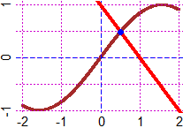
f = function(x) x^2-2; g = function(x) x^3+1
graphF(f, -3,3, "blue"); graph(g, -3,3, "brown")
x = solution2(f,g, -2,0); x; more(x); POINT(x,f(x), "red")
# -1.174559 -1.17455941029298
# K3 You can solve an equation F(x)=G(x) by defining H = F-G and using the command
# solution. But you can also use solution2(F,G, a,b), if the solution is between a and
# b.
f = function(x) x^2-2; g = function(x) x^3+1
graphF(f, -3,3, "blue"); graph(g, -3,3, "brown")
x = solution2(f,g, -2,0); x; more(x); POINT(x,f(x), "red")
# -1.174559 -1.17455941029298
 f = function(x) sin(x); g = function(x) 1-x
graphF(f, -2,2, "brown"); graph(g, -3,3, "red")
z = solution2(f,g, 0,1); more(z); POINT(z,f(z), "blue")
# 0.510973429388569
# You can also refer to WolframAlpha, but the outputs are not always easy to interpret:
# see.
# You can solve the polynomial equations where the only variable that appears is the
# unknown: solution of -78 + 73*x - 57*x^2 + 73*x^3 + 21*x^4 = 0
# [ the coefficients must be set by increasing degrees ]
q = c(-78, 73, -57, 73, 21); solpol(q) [q -> reverse(q) if the order is decreasing]
# 0.857142857142857 -4.33333333333333
# [from the polynomial remainder theorem, we know that a univariate
# polynomial equation of degree N has at most N solutions]
# The outputs are temporarily put into solut (solut[1],solut[2],...)
X = solut; more(X); fraction(X)
# 0.857142857142857 -4.33333333333333
# 6/7 -13/3
# Graphic control (see below to the left):
f = function(x) -78+73*x-57*x^2+73*x^3+21*x^4
graphF(f, -5,2, "blue")
# We can use the command polfun(a,x) to create the function a[1]+a[2]*x+a[3]*x^2+...
g = function(x) polfun(q,x); graphF(g, -5,2, "blue")
# Here's another example: solution of -2/9 - 2/9*x + x^3 + x^4 = 0
# There is no second degree term. I put 0 in place of it.
u = c(-2/9, -2/9, 0, 1, 1); solpol(u)
# 0.60570686427738 -1
f = function(x) -2/9 - 2/9*x + x^3 + x^4
# or:
f = function(x) polfun(u,x)
graphF(f, -1.5,1, "blue")
POINT(solut,c(0,0), "red")
# To get even the complex solutions (see here for complex numbers) instead of solpol we
# use:
u = c(-2/9, -2/9, 0, 1, 1); polyroot(u)
# 0.6057069-0i -0.3028534+0.5245575i -0.3028534-0.5245575i -1+0i
# For more complex polynomial calculations, use Wolframalpha (see). Just that I put:
# quotient and remainder of (x^5 + x^3 - 1) / (x^2 + x - 5)
# to obtain: quotient: x^3 - x^2 + 7*x - 12 remainder: 47*x - 61
# or (x^5 + x^3 - 1) * (x^2 + x - 5) to have:
# x^7 + x^6 - 4*x^5 + x^4 - 5*x^3 - x^2 - x + 5
# or simplify (x^2 + 1) / (x^5 - x) to have: 1/(x^3 - x)
# or lcm x^5 - x, x^2 + 1 to have: (x^2 + 1)*(x^3 - x)
# or gcd x^5 - x, x^2 + 1 to have: x^2 + 1
# [ Here I consider polynomials where a single variable appears. If I consider
# a*x+a*y-y-x like a polynomial of a single indeterminate I must specify what the
# indeterminate is (the concept of "polynomial without indeterminates" does not make
# sense). Here's what happens with WolframAlpha using the Collect command:
# Collect[ a*x+a*y-y-x, a] -> a*(x+y)-x-y, Collect[ a*x+a*y-y-x, x] -> (a-1)*x+a*y-y,
# Collect[ a*x+a*y-y-x, y] -> (a-1)*y+a*x-x. Collect[ u*x^2+u*x+x+u,u] ->
# u*(x^2+x+1)+x, Collect[ u*x^2+u*x+x+u,x] -> u*x^2+(u+1)*x+u. See here, also
# to factorize or expand terms: factor a^2-b^2 -> (a-b)*(a+b),
# expand (a-b)*(a+b) -> a^2-b^2 ]
# You can still add and multiply polynomials with sump and prodp. To work on P =
# x^5 + x^3 - 1 and Q = x^2 + x - 5 you must give the coefficients as input (you need
# to put them by decreasing degree):
P = c(1,0,1,0,0,-1); Q = c(1,1,-5)
# and do this:
sump(P,Q); prodp(P,Q); sump(P,-2*Q) # I have also subtracted from P the double of Q
# 1 0 1 1 1 -6
# 1 1 -4 1 -5 -1 -1 5
# 1 0 1 -2 -2 9
# You obtain: x^5+x^3+x^2+x-6 x^7+x^6-4x^5+x^4-5x^3-x^2-x+5 x^5+x^3-2x^2-2x+9
# If you want use solpol you must reverse the coefficients. The solution of P-2*Q=0:
solpol(reverse(sump(P,-2*Q)))
# -1.3914711989105 the (only) solution of x^5+x^3-2x^2-2x+9=0; ie solpol(c(9,-2,-2,1,0,1))
# To find (x+1)^7 multiply 1 by x+1 7 times:
A = 1; B = c(1,1); for(i in 1:7) A = prodp(A,B); A # "for" -> D-E2
# 1 7 21 35 35 21 7 1
# That is: 1 + 7x + 21x^2 + 35x^3 + 35x^4 + 21x^5 + 7x^6 + x^7
# You can multiply 2, 3, … 8 polynomials with prodp2,…, prodp8. Example:
# (x^5 + x^3 - 1) * (x^2 + x - 5) * (2*x - 1/4)
prodp3(c(1,0,1,0,0,-1),c(1,1,-5),c(2,-1/4))
# 2.00 1.75 -8.25 3.00 -10.25 -0.75 -1.75 10.25 -1.25
fraction(prodp3(c(1,0,1,0,0,-1),c(1,1,-5),c(2,-1/4)))
# 2 7/4 -33/4 3 -41/4 -3/4 -7/4 41/4 -5/4
# ie: 2*x^8 + 7/4*x^7 - 33/4*x^6 + 3*x^5 - 41/4*x^4 - 3/4*x^3 - 7/4*x^2 + 41/4*x - 5/4
#
# With divp you can divide a polynomial by a polynomial. See here.
#
# To repeat a sequence of commands or to modify the execution depending on the value of
# certain variables, use commands: if, ifelse, for, while. It is also often convenient
# to use connectives. Here are some simple examples:
for(i in -2:2) if(i > 0) print(i) # 1 2
for(i in -2:2) if(i >= 0) print(i) # 0 1 2
for(i in -2:2) if(i == 0) print(i) # 0
for(i in -2:2) if(i != 0) print(i) # -2 -1 1 2
for(i in -2:2) if( !(i==0) ) print(i) # -2 -1 1 2
for(i in -2:2) if(i > 0 | i <0) print(i) # -2 -1 1 2
for(i in -2:2) if(i >= 0 & i <= 0) print(i) # 0
for(i in -2:2) if(i == 0) print(i) else print (1/i) # -0.5 -1 0 1 0.5
for(i in -2:2) print( ifelse(i==0, i, 1/i) ) # -0.5 -1 0 1 0.5
for(k in c(1,5,10,50)) print(1/k) # 1 0.2 0.1 0.02
n = 5; k = n; p = 1; while(k > 0) {print(k); p = p*k; k = k-1}; p
# 5 4 3 2 1 120
p = 1; n = 1; while(TRUE) {if(p > 10000) break else {print(p); n=n+1; p = p*n} }
# 1 2 6 24 120 720 5040
p = 1; n = 1; while(! FALSE) {if(p > 10000) break else {print(p); n=n+1; p = p*n} }
# 1 2 6 24 120 720 5040
# { and } allow you to group instructions. Try to understand by yourself what the
# various commands do; then use help("if") help("ifelse") help("&") help("TRUE")
# You can also open from the Help menu the "Html Guide" and then "Packages" (in Windows
# you can open the PDF file "R Reference" that contains a detailed help).
# break allows you to exit from the inside of a "cycle" (or even of the definition of a
# "function").
# In order to signal the end of a long cycle you can introduce the command alarm() which
# gives an audible (or visual, in some platforms) signal to the user.
# Loops (sequences of statements which may be carried out several times, like the ones
# seen above) are the basis of the computer's operation (but they are also the basis of
# every human mathematical activity). An example: the description of an algorithm to
# calculate the reciprocal using only sums, sign change and multiplication, eg 1/7:
f = function(x) sin(x); g = function(x) 1-x
graphF(f, -2,2, "brown"); graph(g, -3,3, "red")
z = solution2(f,g, 0,1); more(z); POINT(z,f(z), "blue")
# 0.510973429388569
# You can also refer to WolframAlpha, but the outputs are not always easy to interpret:
# see.
# You can solve the polynomial equations where the only variable that appears is the
# unknown: solution of -78 + 73*x - 57*x^2 + 73*x^3 + 21*x^4 = 0
# [ the coefficients must be set by increasing degrees ]
q = c(-78, 73, -57, 73, 21); solpol(q) [q -> reverse(q) if the order is decreasing]
# 0.857142857142857 -4.33333333333333
# [from the polynomial remainder theorem, we know that a univariate
# polynomial equation of degree N has at most N solutions]
# The outputs are temporarily put into solut (solut[1],solut[2],...)
X = solut; more(X); fraction(X)
# 0.857142857142857 -4.33333333333333
# 6/7 -13/3
# Graphic control (see below to the left):
f = function(x) -78+73*x-57*x^2+73*x^3+21*x^4
graphF(f, -5,2, "blue")
# We can use the command polfun(a,x) to create the function a[1]+a[2]*x+a[3]*x^2+...
g = function(x) polfun(q,x); graphF(g, -5,2, "blue")
# Here's another example: solution of -2/9 - 2/9*x + x^3 + x^4 = 0
# There is no second degree term. I put 0 in place of it.
u = c(-2/9, -2/9, 0, 1, 1); solpol(u)
# 0.60570686427738 -1
f = function(x) -2/9 - 2/9*x + x^3 + x^4
# or:
f = function(x) polfun(u,x)
graphF(f, -1.5,1, "blue")
POINT(solut,c(0,0), "red")
# To get even the complex solutions (see here for complex numbers) instead of solpol we
# use:
u = c(-2/9, -2/9, 0, 1, 1); polyroot(u)
# 0.6057069-0i -0.3028534+0.5245575i -0.3028534-0.5245575i -1+0i
# For more complex polynomial calculations, use Wolframalpha (see). Just that I put:
# quotient and remainder of (x^5 + x^3 - 1) / (x^2 + x - 5)
# to obtain: quotient: x^3 - x^2 + 7*x - 12 remainder: 47*x - 61
# or (x^5 + x^3 - 1) * (x^2 + x - 5) to have:
# x^7 + x^6 - 4*x^5 + x^4 - 5*x^3 - x^2 - x + 5
# or simplify (x^2 + 1) / (x^5 - x) to have: 1/(x^3 - x)
# or lcm x^5 - x, x^2 + 1 to have: (x^2 + 1)*(x^3 - x)
# or gcd x^5 - x, x^2 + 1 to have: x^2 + 1
# [ Here I consider polynomials where a single variable appears. If I consider
# a*x+a*y-y-x like a polynomial of a single indeterminate I must specify what the
# indeterminate is (the concept of "polynomial without indeterminates" does not make
# sense). Here's what happens with WolframAlpha using the Collect command:
# Collect[ a*x+a*y-y-x, a] -> a*(x+y)-x-y, Collect[ a*x+a*y-y-x, x] -> (a-1)*x+a*y-y,
# Collect[ a*x+a*y-y-x, y] -> (a-1)*y+a*x-x. Collect[ u*x^2+u*x+x+u,u] ->
# u*(x^2+x+1)+x, Collect[ u*x^2+u*x+x+u,x] -> u*x^2+(u+1)*x+u. See here, also
# to factorize or expand terms: factor a^2-b^2 -> (a-b)*(a+b),
# expand (a-b)*(a+b) -> a^2-b^2 ]
# You can still add and multiply polynomials with sump and prodp. To work on P =
# x^5 + x^3 - 1 and Q = x^2 + x - 5 you must give the coefficients as input (you need
# to put them by decreasing degree):
P = c(1,0,1,0,0,-1); Q = c(1,1,-5)
# and do this:
sump(P,Q); prodp(P,Q); sump(P,-2*Q) # I have also subtracted from P the double of Q
# 1 0 1 1 1 -6
# 1 1 -4 1 -5 -1 -1 5
# 1 0 1 -2 -2 9
# You obtain: x^5+x^3+x^2+x-6 x^7+x^6-4x^5+x^4-5x^3-x^2-x+5 x^5+x^3-2x^2-2x+9
# If you want use solpol you must reverse the coefficients. The solution of P-2*Q=0:
solpol(reverse(sump(P,-2*Q)))
# -1.3914711989105 the (only) solution of x^5+x^3-2x^2-2x+9=0; ie solpol(c(9,-2,-2,1,0,1))
# To find (x+1)^7 multiply 1 by x+1 7 times:
A = 1; B = c(1,1); for(i in 1:7) A = prodp(A,B); A # "for" -> D-E2
# 1 7 21 35 35 21 7 1
# That is: 1 + 7x + 21x^2 + 35x^3 + 35x^4 + 21x^5 + 7x^6 + x^7
# You can multiply 2, 3, … 8 polynomials with prodp2,…, prodp8. Example:
# (x^5 + x^3 - 1) * (x^2 + x - 5) * (2*x - 1/4)
prodp3(c(1,0,1,0,0,-1),c(1,1,-5),c(2,-1/4))
# 2.00 1.75 -8.25 3.00 -10.25 -0.75 -1.75 10.25 -1.25
fraction(prodp3(c(1,0,1,0,0,-1),c(1,1,-5),c(2,-1/4)))
# 2 7/4 -33/4 3 -41/4 -3/4 -7/4 41/4 -5/4
# ie: 2*x^8 + 7/4*x^7 - 33/4*x^6 + 3*x^5 - 41/4*x^4 - 3/4*x^3 - 7/4*x^2 + 41/4*x - 5/4
#
# With divp you can divide a polynomial by a polynomial. See here.
#
# To repeat a sequence of commands or to modify the execution depending on the value of
# certain variables, use commands: if, ifelse, for, while. It is also often convenient
# to use connectives. Here are some simple examples:
for(i in -2:2) if(i > 0) print(i) # 1 2
for(i in -2:2) if(i >= 0) print(i) # 0 1 2
for(i in -2:2) if(i == 0) print(i) # 0
for(i in -2:2) if(i != 0) print(i) # -2 -1 1 2
for(i in -2:2) if( !(i==0) ) print(i) # -2 -1 1 2
for(i in -2:2) if(i > 0 | i <0) print(i) # -2 -1 1 2
for(i in -2:2) if(i >= 0 & i <= 0) print(i) # 0
for(i in -2:2) if(i == 0) print(i) else print (1/i) # -0.5 -1 0 1 0.5
for(i in -2:2) print( ifelse(i==0, i, 1/i) ) # -0.5 -1 0 1 0.5
for(k in c(1,5,10,50)) print(1/k) # 1 0.2 0.1 0.02
n = 5; k = n; p = 1; while(k > 0) {print(k); p = p*k; k = k-1}; p
# 5 4 3 2 1 120
p = 1; n = 1; while(TRUE) {if(p > 10000) break else {print(p); n=n+1; p = p*n} }
# 1 2 6 24 120 720 5040
p = 1; n = 1; while(! FALSE) {if(p > 10000) break else {print(p); n=n+1; p = p*n} }
# 1 2 6 24 120 720 5040
# { and } allow you to group instructions. Try to understand by yourself what the
# various commands do; then use help("if") help("ifelse") help("&") help("TRUE")
# You can also open from the Help menu the "Html Guide" and then "Packages" (in Windows
# you can open the PDF file "R Reference" that contains a detailed help).
# break allows you to exit from the inside of a "cycle" (or even of the definition of a
# "function").
# In order to signal the end of a long cycle you can introduce the command alarm() which
# gives an audible (or visual, in some platforms) signal to the user.
# Loops (sequences of statements which may be carried out several times, like the ones
# seen above) are the basis of the computer's operation (but they are also the basis of
# every human mathematical activity). An example: the description of an algorithm to
# calculate the reciprocal using only sums, sign change and multiplication, eg 1/7:
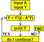 |
A = 7; Y = 0.1         # Y is taken in such a way that A*Y<2
Y = Y*(2-A*Y); more(Y)      # 0.13
Y = Y*(2-A*Y); more(Y)      # 0.1417
Y = Y*(2-A*Y); more(Y)      # 0.14284777
Y = Y*(2-A*Y); more(Y)      # 0.14285714224219
Y = Y*(2-A*Y); more(Y)      # 0.142857142857143
Y = Y*(2-A*Y); more(Y)      # 0.142857142857143
|
# Another command: switch(n, a,b,c,...) is the n-th value in a,b,c,...
switch(4, 1/1, 1/2, 1/3, 1/4, 1/5); switch(4, "H","O","U","S","E")
# 0.25 "S"
# switch(word, p1=X, p2=Y, ...) is X or Y or ... if word is p1 or p2 or ...
who = function(colo) switch(colo, blond="Bea", red="Lia", dark="Rosa"); who("red")
# "Lia"
age = function(name) switch(name, Bea=19,Lia=21,Rosa=22); age("Lia")
# 21
K = c("A","B","C"); K1 = NULL; for(i in 1:3) K1[i]=switch(K[i],"A"=1,"B"=2,"C"=3); K1
# 1 2 3
K2 = NULL; for(i in 1:3) K2[i]=switch(K1[i],"1"="A","2"="B","3"="C"); K2
# "A" "B" "C"
# subset allow you to extract "subsets" from a collection of objects specifying the
# condition that characterizes them.
data = c(118, 135, 127, 119, 121, 124, 130, 132, 128, 122, 121, 123, 127)
data1 = subset(data, data > 120); data2 = subset(data, data-100 > 20 & data-100 < 30)
data1; data2
# 135 127 121 124 130 132 128 122 121 123 127
# 127 121 124 128 122 121 123 127
# An example: the first integer smaller than 10000 with the maximum number of divisors
n=0; for(i in 1:9999) {m=length(divisors(i)); if(m>n) {n=m; j=i}}; c(j,n)
# 7560 64 7560 has 64 divisors; you can see them with divisors(7560)
# ifelse is often used to define functions to be computed in different ways in
# different parts of the domain. A simple example:
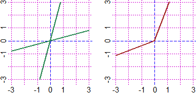
H = function(x) ifelse(x<5, -2, ifelse(x>10, x*2, x) )
# -2 if x < 5, 2x if x > 10, x elsewher, that is in [5,10]
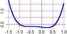
BF=2.5; HF=2; graphF(H, -5, 15, "blue")
 # Here (on the right) another example (a trick to restrict the domain):
K = function(x) ifelse(x >= -1 & x <= 2,abs(-x^2+1),x/0); V = function(x) K(x+1/2)+1
BF=2.5; HF=2; Plane(-2,3, 0,5); graph(K, -2,3, "brown"); graph(V, -2,3, "seagreen")
# The other graphic is obtained with the function DOM, that is 0 if the input belongs
# to the domain of the function FDOM, is not defined otherwise
Plane(-2,3, 0,5); FDOM=K; graph(DOM,-3,3, "brown")
FDOM=V; DOM1 = function(x) DOM(x)+2; graph(DOM1,-2,3, "seagreen")
# DOM is useful to study functions whose domain and range are not known.
# With RANGE (see) we can find the image of a function when input is between 2 values:
RANGE0(K, -1,2)
# "~ min F(min) Max F(Max) mFMF[1:4] = "
# -1 0 2 3 from 0 (in -1) to 3 (in 2)
# I can use the connectives to represent inequalities too (see):
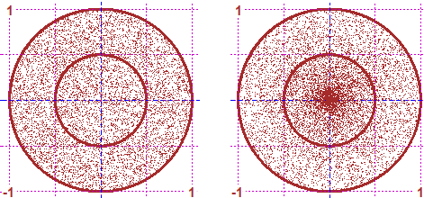
A = function(x,y) 1 <= x^2+y^2
B = function(x,y) (1 <= x^2+y^2 & x^2+y^2 <= 2) | x^2+y^2 <= 0.5
PLANE(-2,2, -2,2); Diseq2(A,0,"seagreen"); POINT(1/2,0, "red")
PLANE(-2,2, -2,2); for(i in 1:10) Diseq2(B,0,"brown"); POINT(1/2,0, "yellow")
A(1/2, 0); B(1/2, 0)
# FALSE TRUE
# Here (on the right) another example (a trick to restrict the domain):
K = function(x) ifelse(x >= -1 & x <= 2,abs(-x^2+1),x/0); V = function(x) K(x+1/2)+1
BF=2.5; HF=2; Plane(-2,3, 0,5); graph(K, -2,3, "brown"); graph(V, -2,3, "seagreen")
# The other graphic is obtained with the function DOM, that is 0 if the input belongs
# to the domain of the function FDOM, is not defined otherwise
Plane(-2,3, 0,5); FDOM=K; graph(DOM,-3,3, "brown")
FDOM=V; DOM1 = function(x) DOM(x)+2; graph(DOM1,-2,3, "seagreen")
# DOM is useful to study functions whose domain and range are not known.
# With RANGE (see) we can find the image of a function when input is between 2 values:
RANGE0(K, -1,2)
# "~ min F(min) Max F(Max) mFMF[1:4] = "
# -1 0 2 3 from 0 (in -1) to 3 (in 2)
# I can use the connectives to represent inequalities too (see):
A = function(x,y) 1 <= x^2+y^2
B = function(x,y) (1 <= x^2+y^2 & x^2+y^2 <= 2) | x^2+y^2 <= 0.5
PLANE(-2,2, -2,2); Diseq2(A,0,"seagreen"); POINT(1/2,0, "red")
PLANE(-2,2, -2,2); for(i in 1:10) Diseq2(B,0,"brown"); POINT(1/2,0, "yellow")
A(1/2, 0); B(1/2, 0)
# FALSE TRUE
 # K4 You can find the minimum degree polynomial whose graph goes through some points
# with the commands: xy_2 (2 points), #&133;, xy_7 (7), xy_fr (fractional form). See.
# From the points: (-2,4) (-1,5) (2,3) (3,-1) (4,-3) (7,4) to the polynomial:
# 211/30 + 341/360*x - 3/2*x^2 - 71/288*x^3 + 37/240*x^4 - 19/1440*x^5
# K4 You can find the minimum degree polynomial whose graph goes through some points
# with the commands: xy_2 (2 points), #&133;, xy_7 (7), xy_fr (fractional form). See.
# From the points: (-2,4) (-1,5) (2,3) (3,-1) (4,-3) (7,4) to the polynomial:
# 211/30 + 341/360*x - 3/2*x^2 - 71/288*x^3 + 37/240*x^4 - 19/1440*x^5
 # You can automatically plot the graph of a 2nd-degree polynomial function and find its
# vertex and focus, with the Parabola and ParabolaM commands: See
# y = -2/3*x^2 + 3*x + 5/3 V: 9/4 121/24 F: 9/4 14/3
# You can automatically plot the graph of a 2nd-degree polynomial function and find its
# vertex and focus, with the Parabola and ParabolaM commands: See
# y = -2/3*x^2 + 3*x + 5/3 V: 9/4 121/24 F: 9/4 14/3
 STATISTICS (and Probability)
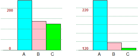
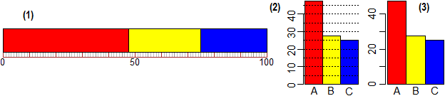
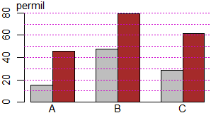
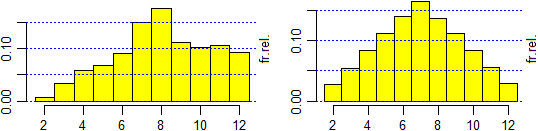
# L-N3 By using BAR2 I can build bar charts that do not start at 0: see here.
STATISTICS (and Probability)
# L-N3 By using BAR2 I can build bar charts that do not start at 0: see here.
 # Note: it is meaningless (although used to fool the reader) to use inclined pie charts.
# See here.
# Besides what we have seen in (L) and (N1), there are many ways to get simply
# bar and circular charts: see here.
# Note: it is meaningless (although used to fool the reader) to use inclined pie charts.
# See here.
# Besides what we have seen in (L) and (N1), there are many ways to get simply
# bar and circular charts: see here.
 # See here for the construction of tables like the following:
 # Let's go deep into what we discussed in (M),(N),(N2),(N3) (and here).
# I can compare boxplots related to a given phenomenon at different times using the
# same scale, if boxAB is assigned the interval in which to plot the boxplot. Example:
# heights of 20-year-old males in 1880 in the intervals of extremes 145,150,…,185 (cm)
# (below 145 and above 185 the percentages are negligible)
freq1 = c(4.0, 6.8, 20.4, 28.4, 23.5, 11.7, 3.7, 1.5)
interv1 = seq(145,185, 5)
BF=4; HF=3; histoclas(interv1,freq1) # see below, on the left
# Let's go deep into what we discussed in (M),(N),(N2),(N3) (and here).
# I can compare boxplots related to a given phenomenon at different times using the
# same scale, if boxAB is assigned the interval in which to plot the boxplot. Example:
# heights of 20-year-old males in 1880 in the intervals of extremes 145,150,…,185 (cm)
# (below 145 and above 185 the percentages are negligible)
freq1 = c(4.0, 6.8, 20.4, 28.4, 23.5, 11.7, 3.7, 1.5)
interv1 = seq(145,185, 5)
BF=4; HF=3; histoclas(interv1,freq1) # see below, on the left
 BF=4; HF=1.4; boxAB = c(145,195); morestat() # see below, the upper boxplot
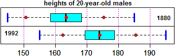 # heights of 20-year-old males in 1992 in the intervals of extremes 155,160,…,195 (cm)
freq2 = c(1.7, 6.8, 18.6, 29.1, 25.2, 13.2, 4.3, 1.1)
interv2 = seq(155,195, 5)
BF=4; HF=3; histoclas(interv2,freq2) # see the histogram on the right
BF=4; HF=1.4; boxAB = c(145,195); morestat()
# see the other boxplot (some writings have been added)
# When you have individual data that can be classified into different intervals it may
# be convenient to represent them with rectangles whose area is the fraction of the
# data falling in the intervals, so that the histogram has a total area of one, as we
# have seen for data already classified in intervals (see here). To do this we use the
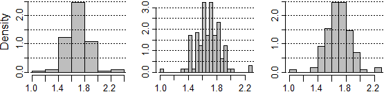
# hist command. Let's see some examples regarding the beans considered in the "part 2".
# dev.new() opens a new device, abline adds grid lines through the current plot.
# [ abline(h=…)/abline(v=…) draw hor./ver. lines; abline(a,b,…) draws the line y=a+b*x
# in the commands abline and plot, lty=3 causes the lines to be dashed, col=… colored,
# lwd=… determines the thickness, ...]
# The number of classes is automatically selected or can be specified, roughly, by
# nclass (or n). With cex.axis I can size the characters. right=FALSE specifies that
# the intervals where the data are classified are of the form […,…).
# The essential thing is: hist(beans, right=FALSE, probability=TRUE).
# "Density" indicates that (on the y axis) the density is represented, that is the
# unitary percentage frequencies (instead of probability=TRUE I can use freq=FALSE).
# [ see here for the unitary percentage frequencies ]
# [ with probability=FALSE or freq=TRUE I get the histogram of the absolute frequencies ]
dev.new()
hist(beans, n=5, right=FALSE, probability=TRUE, cex.axis=0.8, col="grey")
abline(h=axTicks(2),lty=3)
# and what I get with n=20 and with n=10 (or without specifying nclass)
# heights of 20-year-old males in 1992 in the intervals of extremes 155,160,…,195 (cm)
freq2 = c(1.7, 6.8, 18.6, 29.1, 25.2, 13.2, 4.3, 1.1)
interv2 = seq(155,195, 5)
BF=4; HF=3; histoclas(interv2,freq2) # see the histogram on the right
BF=4; HF=1.4; boxAB = c(145,195); morestat()
# see the other boxplot (some writings have been added)
# When you have individual data that can be classified into different intervals it may
# be convenient to represent them with rectangles whose area is the fraction of the
# data falling in the intervals, so that the histogram has a total area of one, as we
# have seen for data already classified in intervals (see here). To do this we use the
# hist command. Let's see some examples regarding the beans considered in the "part 2".
# dev.new() opens a new device, abline adds grid lines through the current plot.
# [ abline(h=…)/abline(v=…) draw hor./ver. lines; abline(a,b,…) draws the line y=a+b*x
# in the commands abline and plot, lty=3 causes the lines to be dashed, col=… colored,
# lwd=… determines the thickness, ...]
# The number of classes is automatically selected or can be specified, roughly, by
# nclass (or n). With cex.axis I can size the characters. right=FALSE specifies that
# the intervals where the data are classified are of the form […,…).
# The essential thing is: hist(beans, right=FALSE, probability=TRUE).
# "Density" indicates that (on the y axis) the density is represented, that is the
# unitary percentage frequencies (instead of probability=TRUE I can use freq=FALSE).
# [ see here for the unitary percentage frequencies ]
# [ with probability=FALSE or freq=TRUE I get the histogram of the absolute frequencies ]
dev.new()
hist(beans, n=5, right=FALSE, probability=TRUE, cex.axis=0.8, col="grey")
abline(h=axTicks(2),lty=3)
# and what I get with n=20 and with n=10 (or without specifying nclass)
 # If you want to add a histogram to an open window, append ,add=TRUE to the options.
# If you do not want to color the inside do not put ,col=…. If you want to color the
# board differently, add ,border=…. To not have the title of the window, add ,main="".
# For more, see the "details".
# To know the height of a histogram (maximum density), for example in the 1st case:
max( hist(beans, nclass=5, right=FALSE, probability=TRUE, plot=FALSE)$density )
# 2.461538
# To know all the absolute or relative frequencies you can use hist(…)$counts or
# hist(…)$density. An example with other data:
da = c(1,2,2,3,3,3,4,4,4,4,5,5,5,5,5,6,7,8,9) # I classify in [0,3), [3,6), [6,10)
A=hist(da,c(0,3,6,10), plot=FALSE,right=FALSE)$counts; A; A/length(da)*100
# 3 12 4 15.78947 63.15789 21.05263
# $ is used to extract outputs from a "command". See here and here for other examples.
# We recall that mean and percentiles for non-classified data are meaningful only if
# the numbers are rounded. For example, if I have numbers truncated to integers I must
# first convert them by adding 1/2 (data = data+1/2); if they are truncated to tenths I
# must add 1/2 tenth (data = data+ 0.1 / 2); if they are truncated to the hundreds I have
# to add 1/2 hundred (data = data + 100/2).
# To simulate (with runif and sample, and set.seed) phenomena and analyze probabilistic
# problems (use of Var, Sd, SdM, study of gaussian and other distributions), and to
# encode/decode messages, see the developments (by the end).
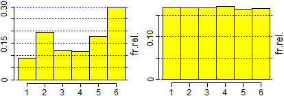
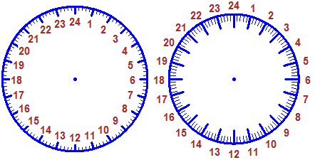
# For an example of random number generation let's see the commands Die(n), DieB(n)
# (that hide the function runif, discussed above). Die(1) and DieB(1) produce the ouput
# of 1 die. Die(N) and DieB(N) with N ≥ 2 produce N outputs and display the distribution
# histogram. One of the two dice is made of wood, the other of thin cardboard, as shown
# below. What are the two dice histograms?
# Test with N≤20000, and evaluate the probability that the output is less than or equal
# to 3 in one case and the other. Which of Die(1) and DieB(1) would you use for a non-
# make-up game?
# Die2(N) and DieB2(N) (with N>1) dispalay the distribution of N outputs of the throw
# of 2 dice. DIE display how to build a die.
# If you want to add a histogram to an open window, append ,add=TRUE to the options.
# If you do not want to color the inside do not put ,col=…. If you want to color the
# board differently, add ,border=…. To not have the title of the window, add ,main="".
# For more, see the "details".
# To know the height of a histogram (maximum density), for example in the 1st case:
max( hist(beans, nclass=5, right=FALSE, probability=TRUE, plot=FALSE)$density )
# 2.461538
# To know all the absolute or relative frequencies you can use hist(…)$counts or
# hist(…)$density. An example with other data:
da = c(1,2,2,3,3,3,4,4,4,4,5,5,5,5,5,6,7,8,9) # I classify in [0,3), [3,6), [6,10)
A=hist(da,c(0,3,6,10), plot=FALSE,right=FALSE)$counts; A; A/length(da)*100
# 3 12 4 15.78947 63.15789 21.05263
# $ is used to extract outputs from a "command". See here and here for other examples.
# We recall that mean and percentiles for non-classified data are meaningful only if
# the numbers are rounded. For example, if I have numbers truncated to integers I must
# first convert them by adding 1/2 (data = data+1/2); if they are truncated to tenths I
# must add 1/2 tenth (data = data+ 0.1 / 2); if they are truncated to the hundreds I have
# to add 1/2 hundred (data = data + 100/2).
# To simulate (with runif and sample, and set.seed) phenomena and analyze probabilistic
# problems (use of Var, Sd, SdM, study of gaussian and other distributions), and to
# encode/decode messages, see the developments (by the end).
# For an example of random number generation let's see the commands Die(n), DieB(n)
# (that hide the function runif, discussed above). Die(1) and DieB(1) produce the ouput
# of 1 die. Die(N) and DieB(N) with N ≥ 2 produce N outputs and display the distribution
# histogram. One of the two dice is made of wood, the other of thin cardboard, as shown
# below. What are the two dice histograms?
# Test with N≤20000, and evaluate the probability that the output is less than or equal
# to 3 in one case and the other. Which of Die(1) and DieB(1) would you use for a non-
# make-up game?
# Die2(N) and DieB2(N) (with N>1) dispalay the distribution of N outputs of the throw
# of 2 dice. DIE display how to build a die.
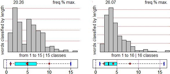
 # By textAnalysis(text) I can analyze the texts statistically. This command does not
# parse the accented letters. If you are in Windows you can use a command with the same
# name (textAnalysis) that also analyzes these characters by loading it with:
source("http://macosa.dima.unige.it/R/textanalysis.R")
# See here for using the command (and maxIsto, maxIstoN, usable to compare histograms
# of different phenomena in the same scale). Here are some of the outputs you get by
# comparing the same piece of "Alice in Wonderland" in Italiano and in English.
# By textAnalysis(text) I can analyze the texts statistically. This command does not
# parse the accented letters. If you are in Windows you can use a command with the same
# name (textAnalysis) that also analyzes these characters by loading it with:
source("http://macosa.dima.unige.it/R/textanalysis.R")
# See here for using the command (and maxIsto, maxIstoN, usable to compare histograms
# of different phenomena in the same scale). Here are some of the outputs you get by
# comparing the same piece of "Alice in Wonderland" in Italiano and in English.
 MORE
# O By using rm(list=ls()) you can remove every definition. Then you must run
# again source("http://macosa.dima.unige.it/r.R")
# rm(v) and rm(v1,v2,...) remove only the variables v, v1, v2, ...
# The warning messages are ignored: if I introduce 5/sqrt(-1)
# I obtain only NaN (it is not a number)
# To print them (as they occur) you must type: options(warn=0). In this case I obtain:
# Warning message: sqrt(-1) NaN
# To deactivate you must type: options(warn=-1)
# It is easy to define sequences by recursion. Three examples (see here for "while"):
# First example: x(1)=1, x(n+1) = ( x(n) + A/x(n) ) / 2 (→ √A)
A=49/9; N=4; x = 1; for (i in 1:N) x = (x+A/x)/2; x
# 2.333335
A=49/9; N=10; x = 1; for (i in 1:N) x = (x+A/x)/2; x
# 2.333333 (L = (L+A/L)/2 -> L^2 = A -> L = √A)
# Second example: u(1) = 1, u(2) = 2, u(n+2) = ( 3*u(n+1)-u(n) )/2
U1 = 1; U2 = 2; N=10; for(i in 3:N) {U = (3*U2-U1)/2; U1 = U2; U2 = U}; U
# 2.996094
U1=1; U2=2; N=20; for(i in 3:N) {U=(3*U2-U1)/2; U1=U2; U2=U}; U
# 2.999996
U1=1; U2=2; N=30; for(i in 3:N) {U=(3*U2-U1)/2; U1=U2; U2=U}; U
# 3 ( If U1=A and U2=A+1 the limit is A+2. Why? )
# Third example: v(1) = 1, v(n+1) = 1+1/v(n)
N=10; x = 1; for (i in 1:N) x = 1+1/x; more(x)
# 1.61797752808989
N=100; x = 1; for (i in 1:N) x = 1+1/x; more(x)
# 1.61803398874989
N=1000; x = 1; for (i in 1:N) x = 1+1/x; more(x)
# 1.61803398874989
# I can find the same value by solving x=1+1/x, ie x^2-x-1=0, for x>0
f=function(x) x^2-x-1; more(solution(f,0, 0,3))
# 1.61803398874989 It is the golden ratio (1+sqrt(5))/2
# Or:
N=100; x = 1; for (i in 1:N) x = sqrt(1+x); more(x)
# 1.61803398874989
# Another example, where I do not proceed by iteration:
exchange = function(x,y) {q=x; x=y; y=q} # I exchange x and y
m=56; p=49; while(p>0){if(p>m) exchange(p,m); k=m; m=p; p=k%%p}; m
# ( I put in order m,n; I replace m with m-n; I replace n with the rest of m/n;
# I get the greatest common divisor of m and n )
# 7
m=4321; p=1234; while(p>0){if(p>m) exchange(p,m); exchange(p,m%%p)}; m
# 1
# I verify using the GCD command:
GCD( c(56,49) ); GCD( c(4321,1234) )
# 7 1
# For a more complex recursive function see here.
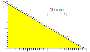
# P-P3 mmpaper allows to create millimeter paper (more freely than mmpaper1/3). Using
# rect for drawing rectangles I can trace histograms too. Examples:
mmpaper(40,25); x = c(1,23,38); y = c(23,9,17); polyline(x,y,"red") # the 1st picture
mmpaper(40,25)
rect(5,0, 10,17, col="red"); rect(10,0, 15,22, col="green") # 5,0 and 10,17 are two
rect(15,0, 20,9, col="blue"); rect(20,0, 25,15, col="cyan") # opposite vertices
rect(25,0, 30,19,col="violet"); rect(30,0, 35,12, col="yellow") # the 2nd picture
MORE
# O By using rm(list=ls()) you can remove every definition. Then you must run
# again source("http://macosa.dima.unige.it/r.R")
# rm(v) and rm(v1,v2,...) remove only the variables v, v1, v2, ...
# The warning messages are ignored: if I introduce 5/sqrt(-1)
# I obtain only NaN (it is not a number)
# To print them (as they occur) you must type: options(warn=0). In this case I obtain:
# Warning message: sqrt(-1) NaN
# To deactivate you must type: options(warn=-1)
# It is easy to define sequences by recursion. Three examples (see here for "while"):
# First example: x(1)=1, x(n+1) = ( x(n) + A/x(n) ) / 2 (→ √A)
A=49/9; N=4; x = 1; for (i in 1:N) x = (x+A/x)/2; x
# 2.333335
A=49/9; N=10; x = 1; for (i in 1:N) x = (x+A/x)/2; x
# 2.333333 (L = (L+A/L)/2 -> L^2 = A -> L = √A)
# Second example: u(1) = 1, u(2) = 2, u(n+2) = ( 3*u(n+1)-u(n) )/2
U1 = 1; U2 = 2; N=10; for(i in 3:N) {U = (3*U2-U1)/2; U1 = U2; U2 = U}; U
# 2.996094
U1=1; U2=2; N=20; for(i in 3:N) {U=(3*U2-U1)/2; U1=U2; U2=U}; U
# 2.999996
U1=1; U2=2; N=30; for(i in 3:N) {U=(3*U2-U1)/2; U1=U2; U2=U}; U
# 3 ( If U1=A and U2=A+1 the limit is A+2. Why? )
# Third example: v(1) = 1, v(n+1) = 1+1/v(n)
N=10; x = 1; for (i in 1:N) x = 1+1/x; more(x)
# 1.61797752808989
N=100; x = 1; for (i in 1:N) x = 1+1/x; more(x)
# 1.61803398874989
N=1000; x = 1; for (i in 1:N) x = 1+1/x; more(x)
# 1.61803398874989
# I can find the same value by solving x=1+1/x, ie x^2-x-1=0, for x>0
f=function(x) x^2-x-1; more(solution(f,0, 0,3))
# 1.61803398874989 It is the golden ratio (1+sqrt(5))/2
# Or:
N=100; x = 1; for (i in 1:N) x = sqrt(1+x); more(x)
# 1.61803398874989
# Another example, where I do not proceed by iteration:
exchange = function(x,y) {q=x; x=y; y=q} # I exchange x and y
m=56; p=49; while(p>0){if(p>m) exchange(p,m); k=m; m=p; p=k%%p}; m
# ( I put in order m,n; I replace m with m-n; I replace n with the rest of m/n;
# I get the greatest common divisor of m and n )
# 7
m=4321; p=1234; while(p>0){if(p>m) exchange(p,m); exchange(p,m%%p)}; m
# 1
# I verify using the GCD command:
GCD( c(56,49) ); GCD( c(4321,1234) )
# 7 1
# For a more complex recursive function see here.
# P-P3 mmpaper allows to create millimeter paper (more freely than mmpaper1/3). Using
# rect for drawing rectangles I can trace histograms too. Examples:
mmpaper(40,25); x = c(1,23,38); y = c(23,9,17); polyline(x,y,"red") # the 1st picture
mmpaper(40,25)
rect(5,0, 10,17, col="red"); rect(10,0, 15,22, col="green") # 5,0 and 10,17 are two
rect(15,0, 20,9, col="blue"); rect(20,0, 25,15, col="cyan") # opposite vertices
rect(25,0, 30,19,col="violet"); rect(30,0, 35,12, col="yellow") # the 2nd picture
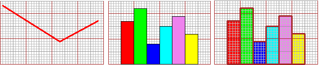 # mmPaper traces the millimeter paper on the same window. The third figure has been
# obtained by these further lines (lwd is the "line width"):
mmPaper(40,25)
rect(5,0, 10,17,border="brown",lwd=3); rect(10,0, 15,22,border="brown",lwd=3)
rect(15,0, 20,9,border="brown",lwd=3); rect(20,0, 25,15,border="brown",lwd=3)
rect(25,0, 30,19,border="brown",lwd=3); rect(30,0, 35,12,border="brown",lwd=3)
# I can add the names of the coordinates using the text command:
mmpaper(100,60)
text(100,-1.7,"100",cex=0.8)
text(0,-1.7,"0",cex=0.8)
text(-2.5,0,"0",cex=0.8,srt=90)
text(-2.5,20,"20",cex=0.8,srt=90)
text(-2.5,60,"60",cex=0.8,srt=90)
Point(0,0, "blue"); Point(100,60, "blue")
line(0,0, 100,60, "blue")
arrow(20*100/60,20, 20*10/6,0, "blue")
arrow(0,20, 20*100/60, 20, "blue")
text(20*10/6,-1.7,"~33",cex=0.8)
# mmPaper traces the millimeter paper on the same window. The third figure has been
# obtained by these further lines (lwd is the "line width"):
mmPaper(40,25)
rect(5,0, 10,17,border="brown",lwd=3); rect(10,0, 15,22,border="brown",lwd=3)
rect(15,0, 20,9,border="brown",lwd=3); rect(20,0, 25,15,border="brown",lwd=3)
rect(25,0, 30,19,border="brown",lwd=3); rect(30,0, 35,12,border="brown",lwd=3)
# I can add the names of the coordinates using the text command:
mmpaper(100,60)
text(100,-1.7,"100",cex=0.8)
text(0,-1.7,"0",cex=0.8)
text(-2.5,0,"0",cex=0.8,srt=90)
text(-2.5,20,"20",cex=0.8,srt=90)
text(-2.5,60,"60",cex=0.8,srt=90)
Point(0,0, "blue"); Point(100,60, "blue")
line(0,0, 100,60, "blue")
arrow(20*100/60,20, 20*10/6,0, "blue")
arrow(0,20, 20*100/60, 20, "blue")
text(20*10/6,-1.7,"~33",cex=0.8)
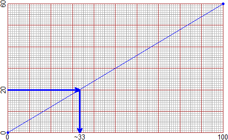 # I can represent circles like the ones below, on the same scale. For details see here
# (the following pictures are reduced).
# I can represent circles like the ones below, on the same scale. For details see here
# (the following pictures are reduced).
 New Sections
S 01 Parametric and Polar Equations. Geometric Transformations
Examples:
New Sections
S 01 Parametric and Polar Equations. Geometric Transformations
Examples:
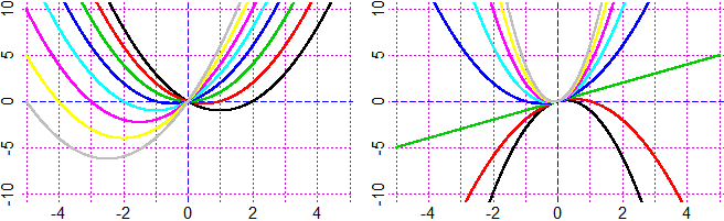 [commands: param polar distPC rottramul multra multiply ... ZZZ; see also #J]
See HERE for the commands (and more).
S 02 Inequalities and Systems of Inequalities (and plane regions)
Examples:
[commands: param polar distPC rottramul multra multiply ... ZZZ; see also #J]
See HERE for the commands (and more).
S 02 Inequalities and Systems of Inequalities (and plane regions)
Examples:
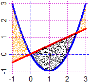
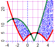
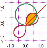
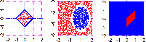
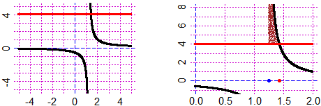 [commands: diseq diseq2 FIGURE ]
See HERE for the commands (and more).
S 03 Vector Calculus
[commands: diseq diseq2 FIGURE ]
See HERE for the commands (and more).
S 03 Vector Calculus
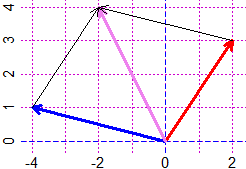 [commands: prodv (or crossp) prods (or dotp) modulus (or magnitude) versor; see also J-2, #J]
See HERE for the commands (and more).
S 04 Lenghts and Areas
[commands: prodv (or crossp) prods (or dotp) modulus (or magnitude) versor; see also J-2, #J]
See HERE for the commands (and more).
S 04 Lenghts and Areas
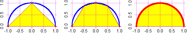 1 1.3660254 1.5707963
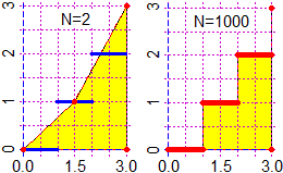
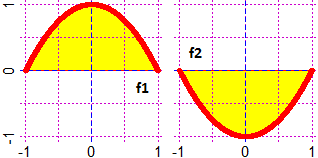 3.75 3 1.333333 -1.333333
| | 3.141593 | 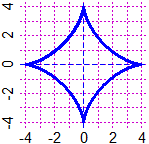 | length = 24
area = 6 π
|
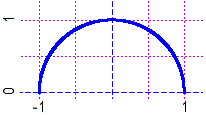 |
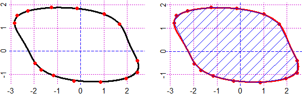 12.8
[commands: areaF areaPar areaPolar lengFun lengPar lengPolar lengPar3 startP x/y Click]
See HERE for the commands (and more).
S 05 Equation systems
12.8
[commands: areaF areaPar areaPolar lengFun lengPar lengPolar lengPar3 startP x/y Click]
See HERE for the commands (and more).
S 05 Equation systems
8x + 7y + 6z = 7.4
7x +10y +12z = 8.65
 x + 2y + 4z = 1.75

x=0.55 y=0.30 z=0.15


                          x=15/13, y=75/13
x=3, y=3 |  |
[commands: eqSystem solut]
See HERE for the commands (and more).
S 06 To estimate the best fit straight line
x: 12±1 17±1 24±1 33±1.5
y: 18±2 27±2 31±2.5 45±3
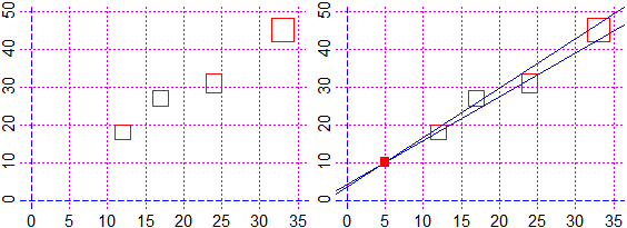 [commands: pointDiff pointDiff0 pointDiff2 colRect rep]
See HERE for the commands (and more).
S 07 Centroid (and Barycenter)
C = centrePol(X,Y); C; POINT(C[1],C[2],"red")
[commands: pointDiff pointDiff0 pointDiff2 colRect rep]
See HERE for the commands (and more).
S 07 Centroid (and Barycenter)
C = centrePol(X,Y); C; POINT(C[1],C[2],"red")
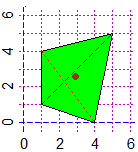
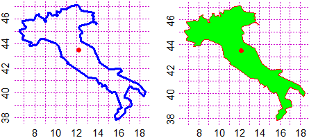 [Centroid coordinates are not the average of X and Y]
[commands: centrePol xTab yTab Line LIne]
See HERE for the commands (and more).
S 08 Integrals and Derivatives (and Limits). Taylor polynomial. Volumes
[Centroid coordinates are not the average of X and Y]
[commands: centrePol xTab yTab Line LIne]
See HERE for the commands (and more).
S 08 Integrals and Derivatives (and Limits). Taylor polynomial. Volumes
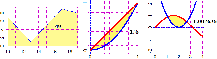

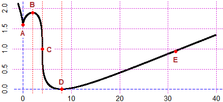
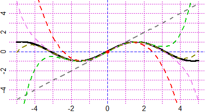 [commands: deriv,deriv2,…,deriv6 derivxy integral Gintegral eval …]
See HERE for the commands (and more).
S 09 Differential equations (1st and 2nd order). Direction fields
y'(x) = x - y(x)
[commands: deriv,deriv2,…,deriv6 derivxy integral Gintegral eval …]
See HERE for the commands (and more).
S 09 Differential equations (1st and 2nd order). Direction fields
y'(x) = x - y(x)
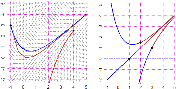 [commands: soledif diredif]
See HERE for the commands (and more).
S 10 Calculations with "big" numbers. Strings <-> Numbers. Bases ≠ ten
x*(10+x)+5*x^3 for x = 123456789012345 -> 9408381861768148891412848380186556157340600
171! -> 124101807021766782342484052410310399261660557750169318538895180361199607522169
175299275197812048758557646495950167038705280988985869071076733124203221848436
431047357788996854827829075454156196485215346831804429323959817369689965723590
3947616152278558180061176365108428800000000000000000000000000000000000000000
as.roman(1944) -> MCMXLIV
MNb(4,100, 2,55) (4/100 in base 2, 55 digits)
0. 0 0 0 0 1 0 1 0 0 0 1 1 1 1 0 1 0 1 1 1 0 0 0 0 1 0 1 0 0
0 1 1 1 1 0 1 0 1 1 1 0 0 0 0 1 0 1 0 0 0 1 1 1 1 remainder 36
## 105!
# 1
# 081
# 39675
# 8240290
# 900504101
# 30580032964
# 9720646107774
# 902579144176636
# 57322653190990515
# 3326984536526808240
# 339776398934872029657
# 99387290781343681609728
# 0000000000000000000000000
[commands: add pro dif app strtoi nchar substr toString NUMBER paste0 as.roman MNb]
See HERE for the commands (and more).
S 11 Perspective. 3D
[commands: soledif diredif]
See HERE for the commands (and more).
S 10 Calculations with "big" numbers. Strings <-> Numbers. Bases ≠ ten
x*(10+x)+5*x^3 for x = 123456789012345 -> 9408381861768148891412848380186556157340600
171! -> 124101807021766782342484052410310399261660557750169318538895180361199607522169
175299275197812048758557646495950167038705280988985869071076733124203221848436
431047357788996854827829075454156196485215346831804429323959817369689965723590
3947616152278558180061176365108428800000000000000000000000000000000000000000
as.roman(1944) -> MCMXLIV
MNb(4,100, 2,55) (4/100 in base 2, 55 digits)
0. 0 0 0 0 1 0 1 0 0 0 1 1 1 1 0 1 0 1 1 1 0 0 0 0 1 0 1 0 0
0 1 1 1 1 0 1 0 1 1 1 0 0 0 0 1 0 1 0 0 0 1 1 1 1 remainder 36
## 105!
# 1
# 081
# 39675
# 8240290
# 900504101
# 30580032964
# 9720646107774
# 902579144176636
# 57322653190990515
# 3326984536526808240
# 339776398934872029657
# 99387290781343681609728
# 0000000000000000000000000
[commands: add pro dif app strtoi nchar substr toString NUMBER paste0 as.roman MNb]
See HERE for the commands (and more).
S 11 Perspective. 3D
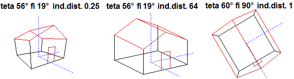

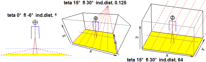 [commands: casa() GRAF3D BOH() seba(0) seba(1) ]
See HERE for the commands (and more).
S 12 Regression. Splines. Curve Fitting. Moving average (or mean).
[commands: casa() GRAF3D BOH() seba(0) seba(1) ]
See HERE for the commands (and more).
S 12 Regression. Splines. Curve Fitting. Moving average (or mean).
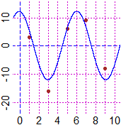
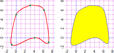
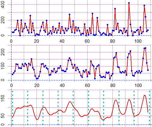 [commands: regression regression1/2/3 spline splineC FRUN…]
See HERE for the commands (and more).
S 13 Bezier curves
[commands: regression regression1/2/3 spline splineC FRUN…]
See HERE for the commands (and more).
S 13 Bezier curves
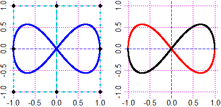 [commands: bezier ]
See HERE for the commands (and more).
S 14 Escher
[commands: bezier ]
See HERE for the commands (and more).
S 14 Escher
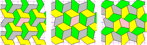 [commands: escher ]
See HERE for the commands (and more).
S 15 Trees and other Graphs
[commands: escher ]
See HERE for the commands (and more).
S 15 Trees and other Graphs
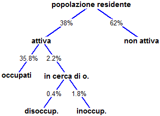
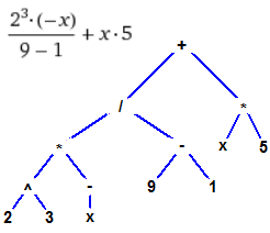
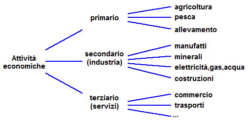

 [commands: PQ Ptext ptext PQtext Ptext2 polyD CLEAN ]
See HERE for the commands (and more).
S 16 Windows without the margins
[commands: PQ Ptext ptext PQtext Ptext2 polyD CLEAN ]
See HERE for the commands (and more).
S 16 Windows without the margins
 [commands: BOXW boxW]
See HERE for the commands (and more).
S 17 Multiple graphs (in the same window)
[commands: BOXW boxW]
See HERE for the commands (and more).
S 17 Multiple graphs (in the same window)

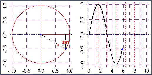
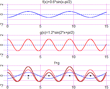 [commands: rowcol colrow Boxm_ Box_ BoxW BoxmW stepline stepl]
See HERE for the commands (and more).
S 18 Animations
[commands: rowcol colrow Boxm_ Box_ BoxW BoxmW stepline stepl]
See HERE for the commands (and more).
S 18 Animations

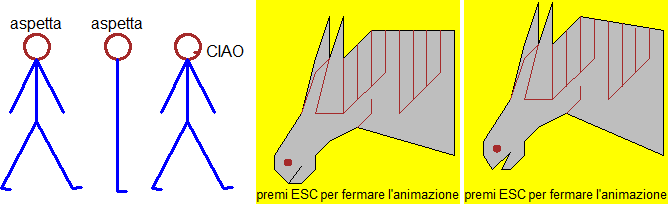
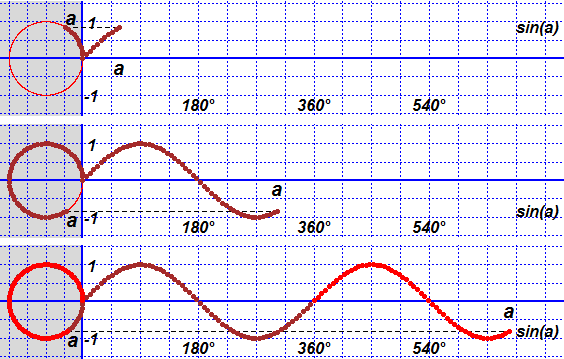
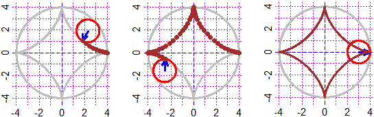 w*sin(x*u)+k*sin(x*v)
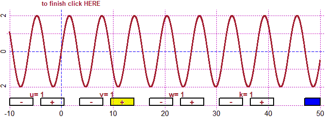
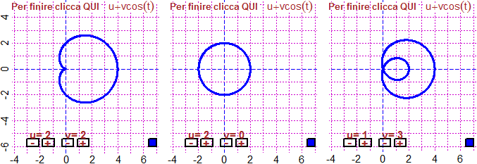
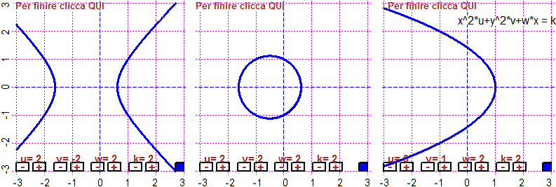
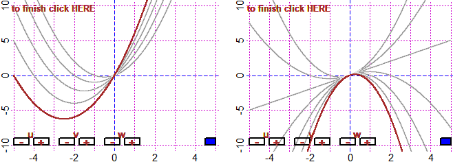 [commands: Hour Minute Second Sec wait BOXw BOXg CLEAN fun3P curve4P polar3P slope]
See HERE for the commands (and more).
S 19 Complex numbers. Matrices. Functions of two variables. Series
[commands: Hour Minute Second Sec wait BOXw BOXg CLEAN fun3P curve4P polar3P slope]
See HERE for the commands (and more).
S 19 Complex numbers. Matrices. Functions of two variables. Series
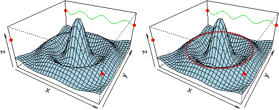
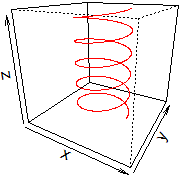
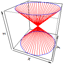
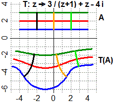
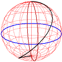
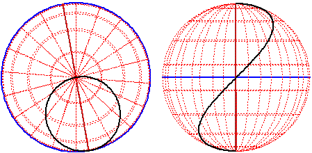
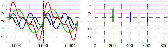 See HERE for the commands (and more).
S 20 Tree structure (and other graphs)
See HERE for the commands (and more).
S 20 Tree structure (and other graphs)
tree( B+C/D*E )

`+`
B
`*`
`/`
C
D
E | 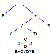  |
[commands: tree (and other commands) ]
See HERE for the commands (and more).
S 21 Random generator of exercises
# An example of how to use runif to randomly generate exercises
x = 3+runif(1)*5+runif(10000)^(runif(1)+0.7)*(runif(1)+5)
BF=4; HF=1.5; statistic(x)
x = 3+runif(1)*5+runif(10000)^(runif(1)+0.7)*(runif(1)+5)
BF=4; HF=1.5; statistic(x)
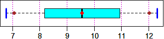
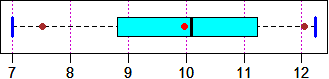 # and to use set.seed to generate specific exercises
set.seed(153); x = 3+runif(1)*5+runif(10000)^(runif(1)+0.7)*(runif(1)+5)
BF=4; HF=1.5; statistic(x)
set.seed(153); x = 3+runif(1)*5+runif(10000)^(runif(1)+0.7)*(runif(1)+5)
BF=4; HF=1.5; statistic(x) # the same exercise, specified by the "seed" 153
# and to use set.seed to generate specific exercises
set.seed(153); x = 3+runif(1)*5+runif(10000)^(runif(1)+0.7)*(runif(1)+5)
BF=4; HF=1.5; statistic(x)
set.seed(153); x = 3+runif(1)*5+runif(10000)^(runif(1)+0.7)*(runif(1)+5)
BF=4; HF=1.5; statistic(x) # the same exercise, specified by the "seed" 153
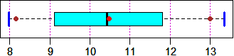 See HERE for the commands (and more).
Command INDEX
Introduction A
> source("http://macosa.dima.unige.it/r.R")
Use as calculator B - E
* / ; .
round sqrt rad2
rad3 fraction …e…
div divisors
Developments E1 - E2
Trees
Here
abs sign rad4/6
%/% quotient remainder
factorial choose Inf .Machine ?Math
round floor e exp print
signif more last
degrees str write
\n \t \b cat for
Other calculi F - G
= c(…) sort
[ ] min max
length sum
Developments G1
-> <-
Here
prod reverse combn
approx approx2 EPS
Figures H - J
PLANE BF HF circle
POINT Point circle3p center3p
radius3p Colors segm
halfline line2p line
point_point inclination angle
mid2p perp2p polyline
leng […:…] polyC
Developments J1 - J6
areaPol xy arrow
dart dirArrow Direction
line_line solut point_inclina
line_line2 noPrint circleA
xrot yrot circle3pA type
circle_circle polylineR polyRC
triLLL triLAL triALA
incentre P_tan
Here
ASP record/replayPlot dev.off
ARC ARCd circl circl3p arc halfl l2p p2p
polyli Ncolor rgb
Quadrilateral P PPP
NW polyS polyS2 text
dart2 arrow2 D… A… bquote Direction
MulTraRot RotTraMul xend yend Dot
Graphs K
Plane abovex abovey
function graph solution
Developments K1 - K3
graphF coldash NpF NPF NpsF
maxmin
Here
underx …X undery U…Y aboveY A… RANGE
PlaneP PLANEP CURVE cur graph1F graph1 …2…
plot distPF CURVEN
TICKx …y Plane2 PLANE2 solution2
solpol solut polyroot sump prodp
if ifelse for while == != | & { } TRUE break subset
Statistics L - N
Bar Pie Strip
ABOVE UNDER above distribution min
max length stem
histogram noClass median
mean Histogram morestat
Developments N1 - N4
BAR BarH PIE PIEh rep Histogram
stem/scale histoclas pointO/D/V
Here (also Probability)
BAR2 BARM PIEH PieC BARC Pie_ … boxAB
hist dev.new abline
nclass cex.axis right=FALSE
runif sample set.seed
Var Sd SdM Die DieB textAnalysis
More O - P
clock GCD primes
LCM Pie(0) gonio(0)
GONIO(0) Strip(0) mmpaper1/2/3
SQUARES INPUT OUTPUT
r/RATIO
Developments P1 - P4
seq : PLANE/W/w/ww Plane/W/w/ww
circleC GRID/w Grid/w gridH/V GridH/V
Gonio CROSS CIRCLE LCROSS COUNT THERMO/2
affine
Here
mmpaper mmPaper CiRcLe dNmM …
New Sections
S01 Parametric and Polar Equations. Geometric Transformations
param polar distCC distPC rottramul multra multiply … ZZZ; see also #J
S02 Inequalities and Systems of Inequalities
diseq diseq2
S03 Vector Calculus
prodv (or crossp) prods (or dotp) modulus (or magnitude) versor; see also J-2, #J
S04 Lenghts and Areas
areaF areaPar areaPolar lengFun lengPar lengPolar lengPar3 startP x/yClick
S05 Equation systems
eqSystem solut
S06 To estimate the best fit straight line
pointDiff pointDiff0 pointDiff2 colRect rep
S07 Centroid (and Barycenter)
centrePol xTab yTab Line LIne
S08 Integrals and Derivatives (and Limits). Taylor polynomial. Volumes
deriv,deriv2,…,deriv6 derivxy integral Gintegral eval …
S09 Differential equations (1st and 2nd order). Direction fields
soledif diredif
S10 Calculations with "big" numbers. Strings <-> Numbers. Bases ≠ ten
add pro dif app strtoi nchar substr toString NUMBER paste0 as.roman MNb
S11 Perspective
casa() GRAF3D BOH() seba(0) seba(1)
S12 Regression. Splines. Curve Fitting. Moving Mean.
regression regression1/2/3 spline
S13 Bezier curves
bezier
S14 Escher
escher
S15 Trees and other Graphs
PQ Ptext ptext PQtext Ptext2 polyD CLEAN
S16 Windows without the margins
BOXW boxW
S17 Multiple graphs (in the same window)
rowcol colrow Boxm_ Box_ BoxW BoxmW stepline stepl
S18 Animations
Hour Minute Second Sec wait BOXw BOXg CLEAN fun3P curve4P polar3P slope
S19 Complex numbers. Matrices. Functions of two variables. Series
[ see the links ]
S20 Tree structure (and other graphs)
tree (and other commands)
S21 Random generator of exercises
The index on a page on its own
See HERE for the commands (and more).
Command INDEX
Introduction A
> source("http://macosa.dima.unige.it/r.R")
Use as calculator B - E
* / ; .
round sqrt rad2
rad3 fraction …e…
div divisors
Developments E1 - E2
Trees
Here
abs sign rad4/6
%/% quotient remainder
factorial choose Inf .Machine ?Math
round floor e exp print
signif more last
degrees str write
\n \t \b cat for
Other calculi F - G
= c(…) sort
[ ] min max
length sum
Developments G1
-> <-
Here
prod reverse combn
approx approx2 EPS
Figures H - J
PLANE BF HF circle
POINT Point circle3p center3p
radius3p Colors segm
halfline line2p line
point_point inclination angle
mid2p perp2p polyline
leng […:…] polyC
Developments J1 - J6
areaPol xy arrow
dart dirArrow Direction
line_line solut point_inclina
line_line2 noPrint circleA
xrot yrot circle3pA type
circle_circle polylineR polyRC
triLLL triLAL triALA
incentre P_tan
Here
ASP record/replayPlot dev.off
ARC ARCd circl circl3p arc halfl l2p p2p
polyli Ncolor rgb
Quadrilateral P PPP
NW polyS polyS2 text
dart2 arrow2 D… A… bquote Direction
MulTraRot RotTraMul xend yend Dot
Graphs K
Plane abovex abovey
function graph solution
Developments K1 - K3
graphF coldash NpF NPF NpsF
maxmin
Here
underx …X undery U…Y aboveY A… RANGE
PlaneP PLANEP CURVE cur graph1F graph1 …2…
plot distPF CURVEN
TICKx …y Plane2 PLANE2 solution2
solpol solut polyroot sump prodp
if ifelse for while == != | & { } TRUE break subset
Statistics L - N
Bar Pie Strip
ABOVE UNDER above distribution min
max length stem
histogram noClass median
mean Histogram morestat
Developments N1 - N4
BAR BarH PIE PIEh rep Histogram
stem/scale histoclas pointO/D/V
Here (also Probability)
BAR2 BARM PIEH PieC BARC Pie_ … boxAB
hist dev.new abline
nclass cex.axis right=FALSE
runif sample set.seed
Var Sd SdM Die DieB textAnalysis
More O - P
clock GCD primes
LCM Pie(0) gonio(0)
GONIO(0) Strip(0) mmpaper1/2/3
SQUARES INPUT OUTPUT
r/RATIO
Developments P1 - P4
seq : PLANE/W/w/ww Plane/W/w/ww
circleC GRID/w Grid/w gridH/V GridH/V
Gonio CROSS CIRCLE LCROSS COUNT THERMO/2
affine
Here
mmpaper mmPaper CiRcLe dNmM …
New Sections
S01 Parametric and Polar Equations. Geometric Transformations
param polar distCC distPC rottramul multra multiply … ZZZ; see also #J
S02 Inequalities and Systems of Inequalities
diseq diseq2
S03 Vector Calculus
prodv (or crossp) prods (or dotp) modulus (or magnitude) versor; see also J-2, #J
S04 Lenghts and Areas
areaF areaPar areaPolar lengFun lengPar lengPolar lengPar3 startP x/yClick
S05 Equation systems
eqSystem solut
S06 To estimate the best fit straight line
pointDiff pointDiff0 pointDiff2 colRect rep
S07 Centroid (and Barycenter)
centrePol xTab yTab Line LIne
S08 Integrals and Derivatives (and Limits). Taylor polynomial. Volumes
deriv,deriv2,…,deriv6 derivxy integral Gintegral eval …
S09 Differential equations (1st and 2nd order). Direction fields
soledif diredif
S10 Calculations with "big" numbers. Strings <-> Numbers. Bases ≠ ten
add pro dif app strtoi nchar substr toString NUMBER paste0 as.roman MNb
S11 Perspective
casa() GRAF3D BOH() seba(0) seba(1)
S12 Regression. Splines. Curve Fitting. Moving Mean.
regression regression1/2/3 spline
S13 Bezier curves
bezier
S14 Escher
escher
S15 Trees and other Graphs
PQ Ptext ptext PQtext Ptext2 polyD CLEAN
S16 Windows without the margins
BOXW boxW
S17 Multiple graphs (in the same window)
rowcol colrow Boxm_ Box_ BoxW BoxmW stepline stepl
S18 Animations
Hour Minute Second Sec wait BOXw BOXg CLEAN fun3P curve4P polar3P slope
S19 Complex numbers. Matrices. Functions of two variables. Series
[ see the links ]
S20 Tree structure (and other graphs)
tree (and other commands)
S21 Random generator of exercises
The index on a page on its own