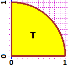
source("http://macosa.dima.unige.it/r.R")    # If I have not already loaded the library
---------- ---------- ---------- ---------- ---------- ---------- ---------- ----------
Integrals of two variables functions
 
# For the integral of a function of two variables (f in [a,b]×[c,d])
# we can use the command  INTEGRAL(f, a,b, c,d, N)  that calculates
# the "volume" of a N×N parallelepiped whose upper part approximates
# the surface of f.
     
  
# When the graph of the function is a plane INTEGRAL approximates very quickly.
# An example:
f = function(x,y) 5
INTEGRAL(f, 0,5, 0,5, 1)
# 125
INTEGRAL(f, 0,5, 0,5, 10)
# 125
# Another (the volume of the part under z=0 equalize the one above):
g = function(x,y) (y-x)/2
INTEGRAL(g, -5,5, -5,5, 1)
# 0
INTEGRAL(f, -5,5, -5,5, 10)
# 0
Other examples:
   
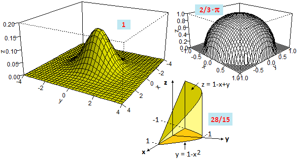
# [1] A bivariate gaussian (just a small N value is enough):
F = function(x,y) 1/(2*pi)*exp(-(x^2+y^2)/2)
u = INTEGRAL(F,-20,20, -20,20, 10); u
# 0.1865616
u = INTEGRAL(F,-20,20, -20,20, 20); u
# 0.9714394
u  =INTEGRAL(F,-20,20, -20,20, 50); u
# 1
#
# [2] The half-sphere of radius 1 (I put 0 out of the domain):
g = function(x,y) ifelse(x^2+y^2>1, 0, sqrt(1-x^2-y^2) )
u = INTEGRAL(g,-1,1, -1,1, 500); u
# 2.094412
u = INTEGRAL(g,-1,1, -1,1, 1000); u
# 2.094397
u/pi
# 0.6666674
fraction(0.6666666666666)
# 2/3  The integral is 2/3·π
#
# [3] The function in the 3rd graph (I put 0 out of the domain):
F = function(x,y) ifelse(y > 1-x^2, 0, 1-x+y)
u = INTEGRAL(F,-1,1, 0,1, 250); more(u)
# 1.86677023999999
u = INTEGR(F,-1,1, 0,1, 500); more(u)
# 1.86705564800002
u = INTEGR(F,-1,1, 0,1, 1000); more(u)
# 1.86669718
fraction(1.866666666666666)
# 28/15
# Using WolframAlpha:
# integrate(integrate 1-x+y, y  =0..1-x^2), x = -1..1
# 28/15
#
# I N is very large, approximation errors can become preponderant.
#
# Another example: integral of (x,y) -> x*y^2 in the following figure
# between y=x^2 and x=y^2

W = function(x,y) ifelse(x>=0 & x<=1 & y>=0 & y<=1 & y^2<=x & y>=x^2, x*y^2, 0)
x1=0; x2=1; y1=0; y2=1; z1=0; z2=1.1
x = seq(x1,x2,len=31); y = seq(y1,y2,len=31); z = outer(x,y,W)
NW(); MARG(0.3); th=0; ph=15
G = persp(x,y,z,zlim=c(z1,z2), theta=th, phi=ph, col="cyan",
      ticktype="detailed",cex.axis=0.75,cex.lab=0.8,d=2)
# The curves that delimit the graph:
t = seq(0,1, len=201); xr=t; yr=xr^2
lines (trans3d(xr, yr, 0, pmat = G), col="red",lwd=2,lty=2)
lines (trans3d(xr, yr, W(xr,yr), pmat=G),col="brown",lwd=3)
t=seq(0,1,len=201); yr=t; xr=yr^2
lines (trans3d(xr, yr, 0, pmat = G), col="red",lwd=2,lty=2)
lines (trans3d(xr, yr, W(xr,yr), pmat = G), col="brown",lwd=3)

# I understand that the integral is much less than 1.
# In the square [0,1]×[0,1] where I have to do the calculation I can simplify
# the function:
Q = function(x,y) ifelse(y^2<=x & y>=x^2, x*y^2, 0)
u1 = INTEGRAL(Q, 0,1, 0,1, 250); more(u1)
#  0.0535951876336641
u2 = INTEGRAL(Q, 0,1, 0,1, 500); more(u2); u1-u2
#  0.0535620065396321   3.318109e-05
u3 = INTEGRAL(Q, 0,1, 0,1, 1000); more(u3); u2-u3
#  0.0535715169843706   -9.510445e-06
# I can stop and take 0.05357. Otherwise:
u4 = INTEGRAL(Q, 0,1, 0,1, 2000); more(u4); u3-u4
#  0.0535723091377355   -7.921534e-07
u5 = INTEGRAL(Q, 0,1, 0,1, 4000); more(u5); u4-u5
#  0.0535716354478788   6.736899e-07
u6 = INTEGRAL(Q, 0,1, 0,1, 8000); more(u6); u5-u6
#  0.0535715329191625   1.025287e-07
# Is it a "fraction"?
fraction(u6)
# 3/56
more(3/56)
# 0.0535714285714286
# If I want, I can use WolframAlpha and verify that 3/56 is actually the exact result
#
# Another example:
# Integral of (x,y) → x^3*y in T.
# I define F so:
F = function(x,y) ifelse(x^2+y^2<=1, x^3*y, 0)
# What is the range of F?
MAXF2(F, 0,1, 0,1)
# ~ max in  x,y  F(max)   0.8675266 0.4973907 0.3247477     
MINF2(F, 0,1, 0,1)
# ~ min in  x,y  F(min)   0.7265506 0.7270941 0.0000000
# From 0 to 0.3; I expect an integral much lower than 1
INTEGRAL(F, 0,1, 0,1, 200)
# 0.04166803
INTEGRAL(F, 0,1, 0,1, 400)
# 0.04166006
INTEGRAL(F, 0,1, 0,1, 800)
# 0.0416674
INTEGRAL(F, 0,1, 0,1, 1600)
# 0.04166695
fraction(0.0416666666666)
# 1/24
#
#
# Another example:
# integral of f in the triangle ->
f = function(x,y) exp((y-x)/(x+y))
PLANE(0,3, 0,3); g = function(x,y) x+y-2; CURVE(g, "brown") 
# I define F so:
F = function(x,y) ifelse(y <= 2-x, f(x,y), 0)
# I put the found values in u:
u = NULL
i=1; u[i] = INTEGRAL(F, 0,2, 0,2, 200); more(u[i])
# 2.35580556893031
i=2; u[i] = INTEGRAL(F,0,2,0,2, 400); more(u[i]); u[i-1]-u[i]
# 2.35287392674027   0.002931642  Subsequent changes will be minor: I can round to 2.35.
# If I want to move forward, I also evaluate the relationship between one variation and the
# next:
i=3; u[i] = INTEGRAL(F,0,2,0,2, 800); more(u[i]); u[i-1]-u[i]; (u[i-2]-u[i-1])/(u[i-1]-u[i])
# 2.35164340648721   0.00123052   2.382441
i=4; u[i] = INTEGRAL(F,0,2,0,2, 1600); more(u[i]); u[i-1]-u[i]; (u[i-2]-u[i-1])/(u[i-1]-u[i])
# 2.35102515514742   0.0006182513   1.990324
i=5; u[i] = INTEGRAL(F,0,2,0,2, 3200); more(u[i]); u[i-1]-u[i]; (u[i-2]-u[i-1])/(u[i-1]-u[i])
# 2.35071560622102   0.0003095489   1.997265
# Taking into account that in this case at every doubling of N the variation is halved, I
# can estimate the distance of the value of the limit equal to the last variation, in fact:
V=1/2; SV=0; for(i in 1:1000) SV=SV+V^i; SV
# 1                                         1/2 + 1/2^2 + 1/2^3 + ... = 1
# Anyway let's move on:
i=6; u[i] = INTEGRAL(F, 0,2, 0,2, 6400); more(u[i]); u[i-1]-u[i]; (u[i-2]-u[i-1])/(u[i-1]-u[i])
# 2.35055913656474   0.0001564697   1.978332
i=7; u[i] = INTEGRAL(F, 0,2, 0,2, 12800); more(u[i]); u[i-1]-u[i]; (u[i-2]-u[i-1])/(u[i-1]-u[i])
# 2.35048072920642   7.840736e-05   1.995599
# The integral is:
2.35048072920642-7.840736e-05; more(2.35048072920642-7.840736e-05)
# 2.350402   2.35040232184642 
# The first rounding is certainly acceptable: 2.350402
# This integral is not trivial, but it is symbolically calculable; you can get:
exp(1)-1/exp(1); more(exp(1)-1/exp(1))
# 2.350402   2.3504023872876
# It is the same value that we have easily found above.
#
# For the graph of two variables functions see S19. 

Other examples of use