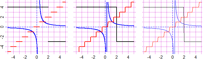
# The graph and graphF commands take quite a long time to plot the 1-input function
# graphs but make them accurate. In the following figure you can see the correct
# graphs of some functions that have jumps made with graph and the wrong ones
# obtained with CURVE and plot, which are discussed below.


# As functions:

f <- function(x) ifelse(x >= 2, -3, 4); g <- function(x) 1/(x-1/3)
h = function(x) round(x)

# As curves:

F <- function(x,y) y - f(x); G <- function(x,y) y - g(x); H = function(x,y) y - h(x)

# 1st:
Plane(-5,5, -5,5); graph(f, -5,5, "black"); graph(g, -5,5, "blue")
graph(h, -5,5, "red")

# 2nd:
Plane(-5,5, -5,5); CURVE(F, "black"); CURVE(G, "blue"); CURVE(H, "red")

# 3rd:
Plane(-5,5, -5,5); plot(f, -5,5, add=TRUE, col="black")
plot(g, -5,5, add=TRUE, col="blue"); plot(h, -5,5, add=TRUE, col="red")
#
# graph and graphF trace the charts by point. If the graph has almost vertical
# sections, it may happen that the curve appears dotted. It may then be useful to
# retract it around those points to get a continuous curve there too. Instead, the
# other commands are almost always trying to match the points that are drawn, as
# seen in the previous figures.
# If I'm sure the function is continuous I can plot the graph with CURVE.

# ["plot" is the standard command for plotting objects; use help("plot") for informations]
#

# GRAPH, GRAPH1, GRAPH2 work like graph, graph1, graph2: they are faster but they draw
# less points. They are good for functions with a graph without sections with high
# slope, as in this case (f, g, h are defined above).

Plane(-5,5,-5,5); GRAPH(f, -5,5, "black"); GRAPH(g, -5,5, "blue"); GRAPH(h, -5,5, "red")
Plane(-5,5,-5,5); GRAPH1(f, -5,5,"black"); GRAPH1(g, -5,5,"blue"); GRAPH1(h, -5,5,"red")
Plane(-5,5,-5,5); GRAPH2(f, -5,5,"black"); GRAPH2(g, -5,5,"blue"); GRAPH2(h, -5,5,"red")
# As functions:
f <- function(x) ifelse(x >= 2, -3, 4); g <- function(x) 1/(x-1/3)
h = function(x) round(x)
# As curves:
F <- function(x,y) y - f(x); G <- function(x,y) y - g(x); H = function(x,y) y - h(x)
# 1st:
Plane(-5,5, -5,5); graph(f, -5,5, "black"); graph(g, -5,5, "blue")
graph(h, -5,5, "red")
# 2nd:
Plane(-5,5, -5,5); CURVE(F, "black"); CURVE(G, "blue"); CURVE(H, "red")
# 3rd:
Plane(-5,5, -5,5); plot(f, -5,5, add=TRUE, col="black")
plot(g, -5,5, add=TRUE, col="blue"); plot(h, -5,5, add=TRUE, col="red")
#
# graph and graphF trace the charts by point. If the graph has almost vertical
# sections, it may happen that the curve appears dotted. It may then be useful to
# retract it around those points to get a continuous curve there too. Instead, the
# other commands are almost always trying to match the points that are drawn, as
# seen in the previous figures.
# If I'm sure the function is continuous I can plot the graph with CURVE.
# ["plot" is the standard command for plotting objects; use help("plot") for informations]
#
# GRAPH, GRAPH1, GRAPH2 work like graph, graph1, graph2: they are faster but they draw
# less points. They are good for functions with a graph without sections with high
# slope, as in this case (f, g, h are defined above).
Plane(-5,5,-5,5); GRAPH(f, -5,5, "black"); GRAPH(g, -5,5, "blue"); GRAPH(h, -5,5, "red")
Plane(-5,5,-5,5); GRAPH1(f, -5,5,"black"); GRAPH1(g, -5,5,"blue"); GRAPH1(h, -5,5,"red")
Plane(-5,5,-5,5); GRAPH2(f, -5,5,"black"); GRAPH2(g, -5,5,"blue"); GRAPH2(h, -5,5,"red")
