source("http://macosa.dima.unige.it/r.R")    # If I have not already loaded the library
---------- ---------- ---------- ---------- ---------- ---------- ---------- ----------
# You can find the minimum degree polynomial whose graph goes through some points
# with the commands:  xy_2(…) (2 points), …, xy_7(…) (7), xy_fr() (fractional form).
# From the points:        (-2,-1)   (6,5)     to the polynomial:
#                           1/2 + 3/4*x
# From the points:     (-1,-2)  (1,4)  (5,0)     to the polynomial:
#                       5/3 + 3*x - 2/3*x^2
# From the points:    (-2,4) (-1,5) (2,3) (3,-1) (4,-3) (7,4)    to the polynomial:
#     211/30 + 341/360*x - 3/2*x^2 - 71/288*x^3 + 37/240*x^4 - 19/1440*x^5
 
       
BF=6; HF=3
Plane(-3,7,-3,8)
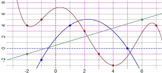
POINT(c(-2,6), c(-1,5), "seagreen")
xy_2(c(-2,6), c(-1,5))
# = function(x) 0.5 + 0.75 *x    Then I define:
f= function(x) 0.5 + 0.75 *x
graph1(f, -4,8, "seagreen")
 
POINT(c(-1,1,5), c(-2,4,0), "blue")
xy_3(c(-1,1,5), c(-2,4,0))
# = function(x) 1.666667 + 3 *x + -0.6666667 *x^2
xy_fr()
#  5/3  3  -2/3    Then I define:
# f= function(x) 1.666667 + 3 *x + -0.6666667 *x^2  or:
f= function(x) 5/3 + 3*x  -2/3*x^2
graph1(f, -4,8, "blue")
 
POINT(c(-2,-1,2,3,4,7), c(4,5,3,-1,-3,4),"brown")
xy_6(c(-2,-1,2,3,4,7), c(4,5,3,-1,-3,4))
# = function(x) 7.033333 + 0.9472222 *x + -1.5 *x^2 + -0.2465278 *x^3 + 0.1541667 *x^4 + -0.01319444 *x^5
xy_fr()
#  211/30  341/360  -3/2  -71/288  37/240 -19/1440        Then I define:
f= function(x) 211/30  + 341/360*x - 3/2*x^2 - 71/288*x^3 + 37/240*x^4 + -19/1440*x^5
graph1(f, -4,8, "brown")

# You can automatically plot the graph of a 2nd-degree polynomial function and find its
# vertex and focus, with the Parabola and ParabolaM commands:
#        y = -2/3*x^2 + 3*x + 5/3      V: 9/4 121/24      F: 9/4 14/3

 
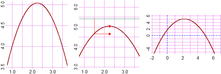# I introduce only the coefficients. The scale and the window are chosen automatically.
# The coordinates of the vertex are printed.
Parabola(-2/3,3,5/3)
# y=a*x^2+b*x+c   V: 2.25 5.041667    [1]  9/4  121/24
 
# I introduce only the coefficients. The monometric scale and the window are chosen
# automatically. The coordinates of the vertex and the focus are printed.
# Vertex, focus and directrix are drown. The points of the parabola are equidistant
# from both the directrix and the focus.
ParabolaM(-2/3,3,5/3)
# y = a*x^2 + b*x + c 
# V: 2.25 5.041667     [1]  9/4  121/24
# F: 2.25 4.666667     [1]  9/4  14/3
 
# The graph with the usual command:
F = function(x) -2/3*x^2+3*x+5/3
Plane(-2,7, -5,6)
graph2(F,-3,8, "brown")

# For the general theme of the conics see here.

Other examples of use