---------- ---------- ---------- ---------- ---------- ---------- ---------- ----------
# The computer, as well as studying large amounts of data, is useful for simulating
# random phenomena. The various programming languages have incorporated a pseudo-random
# number generator. In R there are several random number generators that you can
# explore by typing:
help("RNG") # Random Number Generator
# Let's look at the most commonly used generator in R. Let's first introduce (if we
# have not already introduced it) the following command, which allows us to simplify
# some elaborations.
source("http://macosa.dima.unige.it/r.R")
# The command for this generator is runif, of which we have already seen a first
# explanation here.
#
# runif generates random numbers "uniformly" distributed on the interval (1,10).
# How do I check this out? An initial idea is to check it graphically:
BF=4.5; HF=2.5
Plane(0,1, 0,1.5); hist(runif(1e4),probability=TRUE,nclass=100,add=TRUE,col="grey")
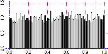 # I can easily verify that as the number of tests increases, the histogram tends to
# flatten. We go from 10 000 to 100 000.
Plane(0,1, 0,1.5); hist(runif(1e5),probability=TRUE,nclass=100,add=TRUE,col="grey")
# I can easily verify that as the number of tests increases, the histogram tends to
# flatten. We go from 10 000 to 100 000.
Plane(0,1, 0,1.5); hist(runif(1e5),probability=TRUE,nclass=100,add=TRUE,col="grey")
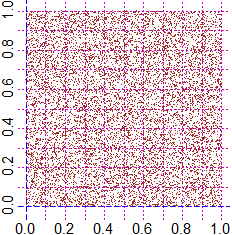
 # It is not enough to see that runif outputs tend to be uniformly distributed. For
# example, if I want to simulate the launch of two dice or the distribution of a hand
# of 10 cards, it is also necessary that an output is independent of the next. The
# study of how to make a random number generator involves many areas of mathematics and
# we can not focus on the topic here. Let's just see, to increase our belief that it's
# a good generator, how are distributed 10000x10000 points generated with it:
BF=3; HF=3
PLANE(0,1, 0,1)
Dot( runif(1e4) ,runif(1e4), "brown")
# It is not enough to see that runif outputs tend to be uniformly distributed. For
# example, if I want to simulate the launch of two dice or the distribution of a hand
# of 10 cards, it is also necessary that an output is independent of the next. The
# study of how to make a random number generator involves many areas of mathematics and
# we can not focus on the topic here. Let's just see, to increase our belief that it's
# a good generator, how are distributed 10000x10000 points generated with it:
BF=3; HF=3
PLANE(0,1, 0,1)
Dot( runif(1e4) ,runif(1e4), "brown")
 # To get an idea of how "runif" is done we see one of the first generators used (1980).
# It displays the functional symbol %% which represents, in R (see here) and in many
# programming languages, the following function:
# mod: (M,N) -> "integer remainder of the division of M by N"
a = 259; M = 65536; x0 = 725; Rand <- function(x) (a*x) %% M
# If I divide by M the results of Rand I get numbers between 0 and 1. Examples:
x = x0
x/M; x = Rand(x); x/M; x = Rand(x); x/M; x = Rand(x); x/M; x = Rand(x); x/M
# 0.01106262 0.8652191 0.0917511 0.7635345 0.7554474
x/M; x = Rand(x); x/M; x = Rand(x); x/M; x = Rand(x); x/M; x = Rand(x); x/M
# 0.7554474 0.6608734 0.166214 0.04942322 0.8006134
# Obviously, a finite number of points is generated: it is a periodic function.
# Let's see what the period is:
alt = 0; n = 1; x = x0
while(alt == 0) if(Rand(x)==x0) {print(n); alt = 1} else {x = Rand(x); n = n+1}
# I get 16384.
# Let's create 3000×3000 points with it. Let's see how they are distributed.
BF=4; HF=4
PLANE(0,1, 0,1); x = x0
for(i in 1:3000) {x = Rand(x); u = x; x = Rand(x); Dot2(u/M, x/M,"brown")}
# To get an idea of how "runif" is done we see one of the first generators used (1980).
# It displays the functional symbol %% which represents, in R (see here) and in many
# programming languages, the following function:
# mod: (M,N) -> "integer remainder of the division of M by N"
a = 259; M = 65536; x0 = 725; Rand <- function(x) (a*x) %% M
# If I divide by M the results of Rand I get numbers between 0 and 1. Examples:
x = x0
x/M; x = Rand(x); x/M; x = Rand(x); x/M; x = Rand(x); x/M; x = Rand(x); x/M
# 0.01106262 0.8652191 0.0917511 0.7635345 0.7554474
x/M; x = Rand(x); x/M; x = Rand(x); x/M; x = Rand(x); x/M; x = Rand(x); x/M
# 0.7554474 0.6608734 0.166214 0.04942322 0.8006134
# Obviously, a finite number of points is generated: it is a periodic function.
# Let's see what the period is:
alt = 0; n = 1; x = x0
while(alt == 0) if(Rand(x)==x0) {print(n); alt = 1} else {x = Rand(x); n = n+1}
# I get 16384.
# Let's create 3000×3000 points with it. Let's see how they are distributed.
BF=4; HF=4
PLANE(0,1, 0,1); x = x0
for(i in 1:3000) {x = Rand(x); u = x; x = Rand(x); Dot2(u/M, x/M,"brown")}
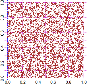 # These graphic outputs are enough to realize the limits of this generator, and the
# complexity of the issue!
#
# Different generators can be used in R. The standard one (which is used in the absence
# of different specifications and dates back to 1998) is periodic (2^19937-1 numbers
# that "repeat" …) and can be used to simulate up to 623 independent events!
# The set.seed(n) command, with n natural number, starts the "random" sequence
# from a given value (with the same n I get the same sequence).
set.seed(7); runif(3); set.seed(7); runif(3)
# 0.9889093 0.3977455 0.1156978 0.9889093 0.3977455 0.1156978
# The "seed" 7 yields, as the first random value, 0.9889093.
# Generating the same sequence of "random" numbers can be convenient in many situations
# (testing an algorithm on the same sequence of values, controlling phenomena
# simulations, memorizing secret encodings, …).
# (incidentally, one of the people who has been busy with random number generators is
# Knuth, the "dad" of the entire "Mathematics of Computing" area that deals with the
# analysis of algorithms; inter alia, in 1978 he invented the typesetting system Teχ)
#
# These graphic outputs are enough to realize the limits of this generator, and the
# complexity of the issue!
#
# Different generators can be used in R. The standard one (which is used in the absence
# of different specifications and dates back to 1998) is periodic (2^19937-1 numbers
# that "repeat" …) and can be used to simulate up to 623 independent events!
# The set.seed(n) command, with n natural number, starts the "random" sequence
# from a given value (with the same n I get the same sequence).
set.seed(7); runif(3); set.seed(7); runif(3)
# 0.9889093 0.3977455 0.1156978 0.9889093 0.3977455 0.1156978
# The "seed" 7 yields, as the first random value, 0.9889093.
# Generating the same sequence of "random" numbers can be convenient in many situations
# (testing an algorithm on the same sequence of values, controlling phenomena
# simulations, memorizing secret encodings, …).
# (incidentally, one of the people who has been busy with random number generators is
# Knuth, the "dad" of the entire "Mathematics of Computing" area that deals with the
# analysis of algorithms; inter alia, in 1978 he invented the typesetting system Teχ)
#