source("http://macosa.dima.unige.it/r.R") # If I have not already loaded the library
---------------------------------------------------------------------------------------
S 01 Parametric and polar equations. Geometric transformations
You can trace curves defined by parametric equations by typing:
param(X,Y, a,b, col) if you have already defined 2 fun. X and Y of a parameter which
varies between a and b, or in polar form with
polar(R, a,b, col) if you have defined R fun. of the angle between a and b
Eg: the following instructions draw an ellipse:
PLANE(-2,2,-2,2)
f <- function(t) 2*cos(t); g <- function(t) sin(t); param(f,g,0,2*pi,'red')
and these draw a spiral:
PLANE(-5,5,-5,5); r <- function(a) sqrt(a); polar(r,0,20,'blue')
With para() par1() pola() pol1() I get a smaller thickness
paramb, polarb, …, pol1b also choose the box, monometric
See below how to draw tangent lines.
To rototranslate the curve K(x,y)=0 of an angle A° around the origin and a vector (h,k)
rottramul(K, A, h,k, mx,my, col)
rottramu(..) rottram(..) They are like "rottramul" but with less thickness
rottra(K, A, h,k, col) It merely rototraslate the curve
To dilate and move the curve and finally rotate it around the origin:
multrarot(K, mx,my, h,k, A, col) multraro(..) multrar(..)
multra(K, mx,my, h,k, col) It merely dilate and traslate the curve
transl(K, h,k, col) traslate
multiply(K, mx,my, col) dilate
We have already seen some examples here.
At each transformation, the transformed curve equation is stored in the ZZZ variable
which, if desired, can be stored with another name and then subjected to other
transformations. To avoid an intermediate curve, we give the color -1 (with the color 0
the curve is dashed).
See here for the use of centrePolar and centreParam to find the centroid (or barycenter)
of a surface described by a polar or a parametric definition (see here for the centroid
of a polygon).
 Examples
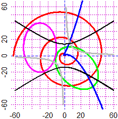
PLANE(-60,60, -60,60)
ro1 <- function(a) a^1.5
polar(ro1,0,5*pi, "red")
ro2 <- function(a) 30/(2+sin(a)-cos(a))
polar(ro2,0,5*pi, "green")
asc1 <- function(t) 2*t^2-3*t
ord1 <- function(t) t^3-t+1
param(asc1, ord1, -10,10, "blue")
asc2 <- function(t) -30+20*cos(t)
ord2 <- function(t) 10+30*sin(t)
param(asc2, ord2, 0,2*pi, "magenta")
H <- function(x,y) x*y-100
CURVE(H, "grey")
rottramu(H, 45, 0,0, 1.5,1, "black")
#
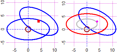
PLANE(-8,12, -5,9)
F <- function(x,y) x^2+y^2-1; CURVE(F,"brown")
multrarot(F, 8,4, 0,0, 0, "blue")
POINT(4,3, "red"); multrarot(F, 8,4, 4,3, -30, "blue")
# figura a destra:
PLANE(-8,12, -5,9)
F <- function(x,y) x^2+y^2-1; CURVE(F,"brown")
multrarot(F, 8,4, 0,0, 0, -1); C1 = ZZZ
POINT(4,3, "magenta"); multrarot(F, 8,4, 4,3, -30, "blue")
multrarot(C1, 1,1, 0,2, 0, "red"); multrarot(C1, 1/2,1/2, 0,2, 0, "grey")
Examples
PLANE(-60,60, -60,60)
ro1 <- function(a) a^1.5
polar(ro1,0,5*pi, "red")
ro2 <- function(a) 30/(2+sin(a)-cos(a))
polar(ro2,0,5*pi, "green")
asc1 <- function(t) 2*t^2-3*t
ord1 <- function(t) t^3-t+1
param(asc1, ord1, -10,10, "blue")
asc2 <- function(t) -30+20*cos(t)
ord2 <- function(t) 10+30*sin(t)
param(asc2, ord2, 0,2*pi, "magenta")
H <- function(x,y) x*y-100
CURVE(H, "grey")
rottramu(H, 45, 0,0, 1.5,1, "black")
#
PLANE(-8,12, -5,9)
F <- function(x,y) x^2+y^2-1; CURVE(F,"brown")
multrarot(F, 8,4, 0,0, 0, "blue")
POINT(4,3, "red"); multrarot(F, 8,4, 4,3, -30, "blue")
# figura a destra:
PLANE(-8,12, -5,9)
F <- function(x,y) x^2+y^2-1; CURVE(F,"brown")
multrarot(F, 8,4, 0,0, 0, -1); C1 = ZZZ
POINT(4,3, "magenta"); multrarot(F, 8,4, 4,3, -30, "blue")
multrarot(C1, 1,1, 0,2, 0, "red"); multrarot(C1, 1/2,1/2, 0,2, 0, "grey")
|
 |  |
( in "polar" it is understood that the angle is in radians; to draw the ro(a) graph
with a in degrees between h and k you must draw that of ro1(x) = ro(x/degrees)
between h/degrees and k/degrees )
# How to calculate the distance of a point from a curve.
# distPC(xP,yP, xt,yt, a,b) calculates the distance between a point
# xP,yP and the curve x=xt(t),y=yt(t) for t from a to b. An example:
PLANE(-8,12, -5,9)
x=function(t) 2+2*cos(t); y=function(t) -1+5*sin(t)
param(x,y, 0,2*pi, "seagreen"); POINT(10,10,"seagreen")
distPC(10,10, x,y, 0,2*pi)
dist. & nearest point (punto piu' vicino):
# 9.644700 2.815577 3.565382
POINT(2.815577,3.565382,"red"); line(2.815577,3.565382,10,10, "red") |
 |
# How to calculate the distance distance between two curves.
# distCC(xt,yt, a,b, ut,vt, c,d) calculates an approximation of the
# distance between two curves: x=xt(t1),y=yt(t1) for t1 from a to b,
# x=ut(t2), y=vt(t2) for t2 from c to d. By narrowing the intervals
# I can improve the accuracy of the approximation. An example:
PLANE(1,6,1,6)
x=function(t) cos(t)*1.5+4.5; y=function(t) sin(t)*1+5
u=function(t) cos(t)+2; v=function(t) sin(t)*1.5+2.5
para(x,y,0,2*pi,"seagreen"); para(u,v,0,2*pi,"seagreen")
distCC(u,v, 0,2*pi, x,y, 0,2*pi)
#  dist.;  t1,t2;  xP,yP,xQ,yQ:
#  0.986040940017622
#  0.9812345  3.7336934
#  2.555997 3.746777  3.255345 4.441895
# I restrict the intervals:
distCC(u,v,0.97,0.99, x,y,3.6,3.9)
#  dist.;  t1,t2;  xP,yP,xQ,yQ:
#  0.986024157784787
#  0.9827379 3.7295597
#  2.554747 3.748029 3.251895 4.445329
distCC(u,v,0.982,0.983, x,y,3.7,3.8)
#  dist.;  t1,t2;  xP,yP,xQ,yQ:
#  0.986024149151057
#  0.9827958 3.7295969
#  2.554698 3.748077 3.251926 4.445298
distCC(u,v,0.9827,0.9828, x,y,3.729,3.73)
#  dist.;  t1,t2;  xP,yP,xQ,yQ:
#  0.986024149136348
#  0.9827937 3.7295952
#  2.554700 3.748075 3.251925 4.445300
# The two curves are 0.98602414914 apart. The nearest points are:
# (2.554700,3.748075) and (3.251926,4.445298) |  |
# Ways to animate geometric transformations are described in S18. A more convenient way
# to draw sheaves of curves is direct use of the following commands, remembering that
# colors can be recalled numerically:
Ncolor()
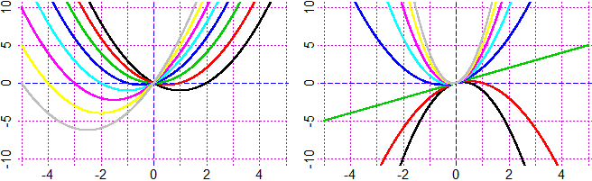
#1 black, 2 red, 3 green, 4 blue, 5 cyan, 6 violet, 7 yellow, 8 grey
h <- function(x) u*x^2+v*x
Plane(-5,5, -10,10) # graphs below to the left (v varies from -2 to 5)
u=1; N = c(-2,-1,0,1,2,3,4,5); for(co in 1:8) {v=N[co]; graph2(h,-5,5,co)}
Plane(-5,5, -10,10) # graphs below to the right (u varies from -2 to 5)
v=1; N = c(-2,-1,0,1,2,3,4,5); for(co in 1:8) {u=N[co]; graph2(h,-5,5,co)}
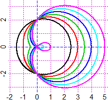
 # If I want to directly draw a sheaf of curves:
ro <- function(t) u+v*cos(t)
#1 black, 2 red, 3 green, 4 blue, 5 cyan, 6 violet
PLANE(-2,5, -3.5,3.5) # v varies in 0.5 1 1.5 ... 3
u=2; N = c(0.5,1,1.5,2,2.5,3); for(co in 1:6) {v=N[co]; pola(ro, 0,2*pi,co)}
# If I want to directly draw a sheaf of curves:
ro <- function(t) u+v*cos(t)
#1 black, 2 red, 3 green, 4 blue, 5 cyan, 6 violet
PLANE(-2,5, -3.5,3.5) # v varies in 0.5 1 1.5 ... 3
u=2; N = c(0.5,1,1.5,2,2.5,3); for(co in 1:6) {v=N[co]; pola(ro, 0,2*pi,co)}
 #1 black, 2 red, 3 green, 4 blue, 5 cyan
BF=4; HF=4
G <- function(x,y) x^2*u+y^2*v+w*x - k
PLANE(-3,3, -3,3) # v varies from -2 to 2
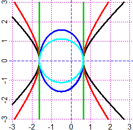
u=2;w=2;k=2; N = c(-2,-1,0,1,2); for(co in 1:5) {v=N[co]; CURVE(G,co)}
#1 black, 2 red, 3 green, 4 blue, 5 cyan
BF=4; HF=4
G <- function(x,y) x^2*u+y^2*v+w*x - k
PLANE(-3,3, -3,3) # v varies from -2 to 2
u=2;w=2;k=2; N = c(-2,-1,0,1,2); for(co in 1:5) {v=N[co]; CURVE(G,co)}
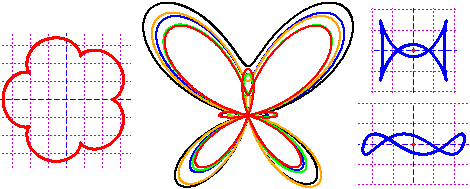
 # Other curves here and here:
 # To find the tangent to the graph of a function you can use "deriv" (see).
# To find the tangent to another curve, it must be of type F(x,y)=0 (see) or it must
# be in parametric or polar form.
# The tangent to a curve in parametric form.
# To find the tangent, in the definition of the curve I have to express the parameter
# by the variable t.
PLANE(-60,60, -60,60)
asc1 <- function(t) 2*t^2-3*t
ord1 <- function(t) t^3-t+1
para(asc1, ord1, -5,5, "blue")
# The point corresponding to t=-2.5
POINT(asc1(-2.5), ord1(-2.5),"seagreen")
d = param_incl(asc1,ord1,-2.5); d
# (inclination of the tangent line when t=-2.5)
# -53.78116
point_incl(asc1(-2.5),ord1(-2.5), d, "black")
# (point_incl(x,y,d): line through x,y with inclination d)
# To find the tangent to the graph of a function you can use "deriv" (see).
# To find the tangent to another curve, it must be of type F(x,y)=0 (see) or it must
# be in parametric or polar form.
# The tangent to a curve in parametric form.
# To find the tangent, in the definition of the curve I have to express the parameter
# by the variable t.
PLANE(-60,60, -60,60)
asc1 <- function(t) 2*t^2-3*t
ord1 <- function(t) t^3-t+1
para(asc1, ord1, -5,5, "blue")
# The point corresponding to t=-2.5
POINT(asc1(-2.5), ord1(-2.5),"seagreen")
d = param_incl(asc1,ord1,-2.5); d
# (inclination of the tangent line when t=-2.5)
# -53.78116
point_incl(asc1(-2.5),ord1(-2.5), d, "black")
# (point_incl(x,y,d): line through x,y with inclination d)
 # The tangent to a curve in polar form (image on the right).
# To find the tangent, in the definition of the curve I have to express the angle
# by the variable ang.
PLANE(-60,60, -60,60)
ro1 = function(ang) ang^1.5
pola(ro1, 0,5*pi, "red")
# The point corresponding to ang of 450°
a=450/180*pi; x=ro1(a)*cos(a);y=ro1(a)*sin(a); POINT(x,y,"blue")
d = polar_incl(ro1,a); d
# -10.81248
point_incl(x,y, d, "brown")
# (point_incl(x,y,d): line through x,y with inclination d)
Other examples of use
# The tangent to a curve in polar form (image on the right).
# To find the tangent, in the definition of the curve I have to express the angle
# by the variable ang.
PLANE(-60,60, -60,60)
ro1 = function(ang) ang^1.5
pola(ro1, 0,5*pi, "red")
# The point corresponding to ang of 450°
a=450/180*pi; x=ro1(a)*cos(a);y=ro1(a)*sin(a); POINT(x,y,"blue")
d = polar_incl(ro1,a); d
# -10.81248
point_incl(x,y, d, "brown")
# (point_incl(x,y,d): line through x,y with inclination d)
Other examples of use