source("http://macosa.dima.unige.it/r.R") # If I have not already loaded the library
---------- ---------- ---------- ---------- ---------- ---------- ---------- ----------
S 05 Equation systems
eqSystem(x) solves the linear system x
solut[n] is the n-th solution (if before "eqSystem" I put noPrint=1, the solutions are
# not printed and can only be seen with the solut command).
## (I have three metal bars made of silver, copper and tin. Their compositions are:
## silver copper tin
## 1^ 80% 17.5% 2.5% How much metal do you need to take from each bar to get
## 2^ 70% 25% 5% a compound metal in the following way?
## 3^ 60% 30% 10% silver: 74% copper: 21.625% tin: 4.375%
## Let's solve the system
# 80x + 70y + 60z = 74
# 17.5x + 25y + 30z = 21.625
# 2.5x + 5y + 10z = 4.375
S = c(
80,70,60, 74,
17.5,25,30, 21.625,
2.5, 5,10, 4.375 )
eqSystem(S)
# 0.55 0.30 0.15
solut[2] # To display only the 2nd solution (y)
# 0.3
## 55% must be taken from the first bar, 30% from the second, 15% from the third
# If the system has no solution or has infinitely many solutions it appears "singular
# system".
# The intersection of the three planes x-y-4z=3, x+y-2z=1, 3x+6y-z=0
Q = c(1,-1,-4,3, 1,1,-2,1, 3,6,-1,0); eqSystem(Q)
# 2 -1 0
# The point of intersection is (2,-1,0)
# Another example. The linear system:
# 2x-5y+4z+ u = -3
# x-2y+ z- u = 5
# x+ 6z+2u = 10
# 12x+4y+3z = 2
S = c(
2,-5, 4, 1, -3,
1,-2, 1,-1, 5,
1, 0, 6, 2, 10,
12, 4, 3, 0, 2)
eqSystem(S)
# -1.496599 1.959184 4.040816 -6.374150
fraction(solut[1:4])
# -220/147 96/49 198/49 -937/147
#
# For nonlinear systems, you can go graphically and find solutions up to 6 or 7 digits.
# But when you can relate to an equation in one variable, you can use equation
# resolution. Let's see a simple example:
# Find the intersections between 2y+3x-15=0 (line) and (x-3)^2+(y-5)^2=4 (circle)
f = function(x) (15-3*x)/2; g = function(x,y) (x-3)^2+(y-5)^2-4
PLANE(0,7, 0,7); CURVE(g, "blue"); graph( f, 0,7, "blue")
# I get the chart below to the left:
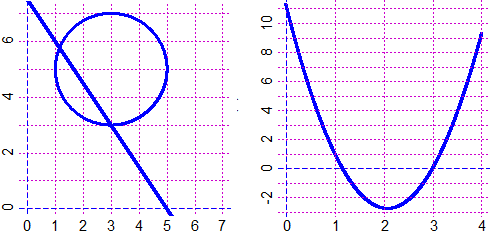 # To find the intersections I consider:
h = function(x) g(x, f(x)); graphF( h, 0,4, "blue")
# [ h(x)=0 when f(x)=y and g(x,y)=0 ]
# I get the chart above to the right, where I see the "x" solutions better
solution(h,0, 0,2)
# 1.153846
more(solution(h,0, 0,2))
# 1.15384615384615
fraction(solution(h,0, 0,2))
# 15/13
solution(h,0, 2,4)
# 3
# The x are 15/13 and 3, I find the y:
f(15/13); f(3)
# 5.769231 3
fraction( f(15/13) )
# 75/13
# The solutions are (x,y) = (15/13, 75/13) and (x,y) = (3,3), which I can control on
# the graph above, on the left
Other examples of use
# To find the intersections I consider:
h = function(x) g(x, f(x)); graphF( h, 0,4, "blue")
# [ h(x)=0 when f(x)=y and g(x,y)=0 ]
# I get the chart above to the right, where I see the "x" solutions better
solution(h,0, 0,2)
# 1.153846
more(solution(h,0, 0,2))
# 1.15384615384615
fraction(solution(h,0, 0,2))
# 15/13
solution(h,0, 2,4)
# 3
# The x are 15/13 and 3, I find the y:
f(15/13); f(3)
# 5.769231 3
fraction( f(15/13) )
# 75/13
# The solutions are (x,y) = (15/13, 75/13) and (x,y) = (3,3), which I can control on
# the graph above, on the left
Other examples of use