source("http://macosa.dima.unige.it/r.R") # If I have not already loaded the library
---------- ---------- ---------- ---------- ---------- ---------- ---------- ----------
S 06 To estimate the best fit straight line
Straight line that crosses exactly (A,B) and fits some points that have x and y
coordinates with ex and ey precisions. Command:
pointDiff(A,B, x,y, ex,ey)
pointDiff2(A,B, x,y, ex,ey) produces outputs in fractional form
Instead, if I use the following command I represent points without curves that
approximate them.
pointDiff0(x,y, ex,ey)
# I can change color to the rectangles that represent points with colRect command.
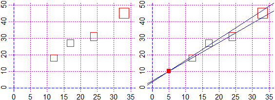
# What can I say about the linear function F such that F(5) = 10 whose graph passes
# through:
# x: 12±1 17±1 24±1 33±1.5
# y: 18±2 27±2 31±2.5 45±3
Plane(0,35, 0,50)
x = c(12, 17, 24, 33); ex = c(1, 1, 1, 1.5)
y = c(18, 27, 31, 45); ey = c(2, 2, 2.5, 3)
pointDif(5,10, x,y, ex,ey)
# 1.153846 * x + 4.230769 1.153846 * (x - 5 ) + 10
# 1.305556 * x + 3.472222 1.305556 * (x - 5 ) + 10
# I get the figure below on the right:
 # If I wanted to express the values in fractional:
pointDif2(5,10, x,y, ex,ey)
# 15/13 55/13 15/13 5 10 47/36 125/36 47/36 5 10
# I deduce: 15/13*x+55/13 15/13*(x-5)+10 47/36*x+125/36 47/36*(x-5)+10
# If I want to plot the points with their precision without approximating them with a
# straight line, I use the following command, getting the figure above on the left:
pointDif0(x,y, ex,ey)
# If before these commands I put, for example, colRet="brown", the rectangles would
# be drawn in brown.
# If the precisions are all the same, if (for example) the points are N and ex are
# all 2, I can put ex = rep(2,N).
Other examples of use
# If I wanted to express the values in fractional:
pointDif2(5,10, x,y, ex,ey)
# 15/13 55/13 15/13 5 10 47/36 125/36 47/36 5 10
# I deduce: 15/13*x+55/13 15/13*(x-5)+10 47/36*x+125/36 47/36*(x-5)+10
# If I want to plot the points with their precision without approximating them with a
# straight line, I use the following command, getting the figure above on the left:
pointDif0(x,y, ex,ey)
# If before these commands I put, for example, colRet="brown", the rectangles would
# be drawn in brown.
# If the precisions are all the same, if (for example) the points are N and ex are
# all 2, I can put ex = rep(2,N).
Other examples of use