source("http://macosa.dima.unige.it/r.R") # If I have not already loaded the library
---------- ---------- ---------- ---------- ---------- ---------- ---------- ----------
S 08 Integrals and Derivatives (and Limits). Taylor polynomial. Volumes.
# deriv(f,VariableName), deriv2, …, deriv6
# Note: deriv(f,"a") equals D(body(f),"a")
G = function(u) sin(u); deriv(G,"u")
# cos(u)
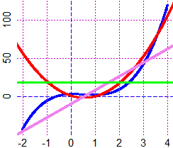
f = function(x) 3*x^3-5*x^2+x+3
graphF(f, -2,4, "blue")
deriv(f,"x")
# 3 * (3 * x^2) - 5 * (2 * x) + 1
# To use the expression produced by "deriv" you need to evaluate it with eval:
df = function(x) eval(deriv(f,"x"))
graph(df,-3,5, "red")
# I could also define df by writing 3*(3*x^2)-5*(2*x)+1 [ or 9*x^2-10*x+1 ]
deriv2(f,"x")
# 3 * (3 * (2 * x)) - 5 * 2
d2f = function(x) eval(deriv2(f,"x")); graph(d2f,-3,5, "violet")
deriv3(f,"x")
# 3 * (3 * 2)
d3f = function(x) eval(deriv3(f,"x"))+x-x # I put the "x" with a trick
graph(d3f,-3,5, "green")
 # To evaluate the derivative of log10(x) and log2(x) you must use log(x)/log(10) and
# log(x)/log(2), where log(x) is the inverse of exp(x)
f=function(x) log(x); g=function(x) log(x)/10; h=function(x) log(x)/2
deriv(f,"x"); deriv(g,"x"); deriv(h,"x")
# 1/x 1/x/10 1/x/2
# To evaluate the derivative of a function where abs(u) appears, it needs to be
# replaced with sqrt(u^2)
#
# If f is a piecewise-defined function we must derive every sub-function (see).
# To evaluate the derivative of log10(x) and log2(x) you must use log(x)/log(10) and
# log(x)/log(2), where log(x) is the inverse of exp(x)
f=function(x) log(x); g=function(x) log(x)/10; h=function(x) log(x)/2
deriv(f,"x"); deriv(g,"x"); deriv(h,"x")
# 1/x 1/x/10 1/x/2
# To evaluate the derivative of a function where abs(u) appears, it needs to be
# replaced with sqrt(u^2)
#
# If f is a piecewise-defined function we must derive every sub-function (see).
 #
# Note. df calculated by the software can have a wider domain than f. Example:
#
# Note. df calculated by the software can have a wider domain than f. Example:
 f = function(x) log(1+tan(x/2))
BF=5; HF=3; a=-2*pi; b=2*pi; Plane(a,b, -5,5)
graph2(f, a,b, "brown"); df = function(x) eval( deriv(f,"x") ); deriv(f,"x")
# 1/2/cos(x/2)^2/(1 + tan(x/2))
graph2(df, a,b, "seagreen")
FDOM=f; graph(DOM, a,b, "red") # DOM is defined 0 in the domain of FDOM
pointO(pi*c(-1,-1/2,1,2-1/2),rep(0,4),"blue")
text(-5,-1/2,"domain",font=2,col="red"); text(-1/2,-1.5,"f",font=2,col="brown")
text(-1/2,2.5,"df",font=2,col="seagreen"); text(-2.5,-1.5,"?",font=2,col="seagreen")
#
# I can calculate the integral of a piecewise linear function (with coordinates in x
# and y), using the areaPol command, if I define:
INTEGRAL = function(x,y) areaPol( c(x[length(x)],x[1],x), c(0,0,y) )
# Example:
f = function(x) log(1+tan(x/2))
BF=5; HF=3; a=-2*pi; b=2*pi; Plane(a,b, -5,5)
graph2(f, a,b, "brown"); df = function(x) eval( deriv(f,"x") ); deriv(f,"x")
# 1/2/cos(x/2)^2/(1 + tan(x/2))
graph2(df, a,b, "seagreen")
FDOM=f; graph(DOM, a,b, "red") # DOM is defined 0 in the domain of FDOM
pointO(pi*c(-1,-1/2,1,2-1/2),rep(0,4),"blue")
text(-5,-1/2,"domain",font=2,col="red"); text(-1/2,-1.5,"f",font=2,col="brown")
text(-1/2,2.5,"df",font=2,col="seagreen"); text(-2.5,-1.5,"?",font=2,col="seagreen")
#
# I can calculate the integral of a piecewise linear function (with coordinates in x
# and y), using the areaPol command, if I define:
INTEGRAL = function(x,y) areaPol( c(x[length(x)],x[1],x), c(0,0,y) )
# Example:
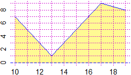 x = c(10,13, 17, 19); y = c(7,1,9,8)
Plane(min(x),max(x), 0,max(y)); polyl(x,y,"blue")
INTEGRAL = function(x,y) areaPol( c(x[length(x)],x[1],x), c(0,0,y) )
INTEGRAL(x,y)
# 49
# We can use areaPol also for spline functions (see):
x = c(-0.2, 1.3, 1.7, 3.2, 4.1, 4.6)
y = c(9.1, 17.5, 20.7, 25.4, 35.7, 51.2)
Plane(-1,6,-10,70); POINT(x,y,1); L=spline(x,y,1000); polyline(L$x,L$y,"red")
INTEGRAL(L$x,L$y) # INTEGRAL defined above
# 108.6348
x = c(10,13, 17, 19); y = c(7,1,9,8)
Plane(min(x),max(x), 0,max(y)); polyl(x,y,"blue")
INTEGRAL = function(x,y) areaPol( c(x[length(x)],x[1],x), c(0,0,y) )
INTEGRAL(x,y)
# 49
# We can use areaPol also for spline functions (see):
x = c(-0.2, 1.3, 1.7, 3.2, 4.1, 4.6)
y = c(9.1, 17.5, 20.7, 25.4, 35.7, 51.2)
Plane(-1,6,-10,70); POINT(x,y,1); L=spline(x,y,1000); polyline(L$x,L$y,"red")
INTEGRAL(L$x,L$y) # INTEGRAL defined above
# 108.6348
 # But I can use the integral(f, a,b) command, if I define such function explicitly:
f = function(x) ifelse(x<13, 7-6/3*(x-10), ifelse(x<17, 1+8/4*(x-13), 9-1/2*(x-17)))
Plane(10,19, 0,9); graph(f, 10,19, "blue")
# But I can use the integral(f, a,b) command, if I define such function explicitly:
f = function(x) ifelse(x<13, 7-6/3*(x-10), ifelse(x<17, 1+8/4*(x-13), 9-1/2*(x-17)))
Plane(10,19, 0,9); graph(f, 10,19, "blue")
 integral(f, 10,19)
# 49
# A function that can be described more easily:
g = function(x) sin(x)
integral(sin, 0,pi/2); integral(sin, 0,pi); integral(sin, 0,2*pi)
# 1 2 2.032977e-16 ("pratically" 0)
# Here, how to calculate the effective force on the mast of a racing sailbot
# (from "Numerical Methods", Chapra & Canale, McGraw-Hill)
integral(f, 10,19)
# 49
# A function that can be described more easily:
g = function(x) sin(x)
integral(sin, 0,pi/2); integral(sin, 0,pi); integral(sin, 0,2*pi)
# 1 2 2.032977e-16 ("pratically" 0)
# Here, how to calculate the effective force on the mast of a racing sailbot
# (from "Numerical Methods", Chapra & Canale, McGraw-Hill)
 # See here for integrals of F from A to B when A or B are infinite or F is undefined
# at A or B .
# Definite integrals of many funcions can be calculated with the areaF command: see.
# Only when we have focused the theorem fundamental theorem of calculus (see here or
# here) we can interpret areas as defined integrals.
#
# Gintegral(f,A,B,col) traces the graph of x -> ∫[A,x]f from A to B (A and B must be
# finite); Gintegra, Gintegr plot slimmer graphics.
Plane(-pi,2*pi, -1,1); graph1(cos, -pi,2*pi, "blue")
Gintegr(cos, 0,2*pi, "red"); Gintegr(cos, 0,-pi, "violet")
POINT(0,0, "red")
# See here for integrals of F from A to B when A or B are infinite or F is undefined
# at A or B .
# Definite integrals of many funcions can be calculated with the areaF command: see.
# Only when we have focused the theorem fundamental theorem of calculus (see here or
# here) we can interpret areas as defined integrals.
#
# Gintegral(f,A,B,col) traces the graph of x -> ∫[A,x]f from A to B (A and B must be
# finite); Gintegra, Gintegr plot slimmer graphics.
Plane(-pi,2*pi, -1,1); graph1(cos, -pi,2*pi, "blue")
Gintegr(cos, 0,2*pi, "red"); Gintegr(cos, 0,-pi, "violet")
POINT(0,0, "red")
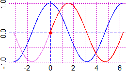
 # The graph on the right:
Plane(-pi,2*pi, -1,1); graph1(cos, -pi,2*pi, "blue")
POINT(2.5,0.5, "red")
GintegrK(cos, 2.5,2*pi, 0.5, "brown"); GintegrK(cos, 2.5,-pi, 0.5, "seagreen")
# With GintegralK(f,A,B, k, col) (and GintegraK, GintegrK) I can trace the graph
# of x -> k + ∫[A,x]f
# In very special cases Gintegral (Gintegra, Gintegr) may not work; in such cases you
# can try using GintegralA or, if it is not working, GintegralB or … GintegralD, or
# Gintegral0 (or GintegraA, GintegrA, … Gintegra0, Gintegr0, for slimmer graphics):
f = function(x) ifelse(x<13, 7-6/3*(x-10), ifelse(x<17, 1+8/4*(x-13), 9-1/2*(x-17)))
Plane(10,19, 0,50); Gintegra(f, 10,19, "blue")
# Error in integrate
Plane(10,19, 0,50); GintegraA(f, 10,19, "brown")
# The graph on the right:
Plane(-pi,2*pi, -1,1); graph1(cos, -pi,2*pi, "blue")
POINT(2.5,0.5, "red")
GintegrK(cos, 2.5,2*pi, 0.5, "brown"); GintegrK(cos, 2.5,-pi, 0.5, "seagreen")
# With GintegralK(f,A,B, k, col) (and GintegraK, GintegrK) I can trace the graph
# of x -> k + ∫[A,x]f
# In very special cases Gintegral (Gintegra, Gintegr) may not work; in such cases you
# can try using GintegralA or, if it is not working, GintegralB or … GintegralD, or
# Gintegral0 (or GintegraA, GintegrA, … Gintegra0, Gintegr0, for slimmer graphics):
f = function(x) ifelse(x<13, 7-6/3*(x-10), ifelse(x<17, 1+8/4*(x-13), 9-1/2*(x-17)))
Plane(10,19, 0,50); Gintegra(f, 10,19, "blue")
# Error in integrate
Plane(10,19, 0,50); GintegraA(f, 10,19, "brown")
 # For the same reasons if integral does not work you can use integralA, …, intergralD
# or intergral0.
#
# In some case, some manipulations are necessary to achieve a result: a simple example.
#
# With R we can compute definite integrals. We can also calculate the indefinite
# integrals (ie antiderivatives) of polynomial functions.
Q = c(-2,-3,2.4,-1/5) # the polynomial -2-3*x+2.4*x^2-1/5*x^3
q = function(x) Q[1]+x*Q[2]+x^2*Q[3]+x^3*Q[4]
# the integral:
I = function(p) {I=NULL; for (i in 1:length(p)) I = c(I,p[i]/i); I}
I(Q); fraction(I(Q))
# -2.00 -1.50 0.80 -0.05
# -2 -3/2 4/5 -1/20 -2*x-3/2*x^2+4/5*x^3-1/20*x^4 + constant
Iq = function(x) x*I(Q)[1]+x^2*I(Q)[2]+x^3*I(Q)[3]+x^4*I(Q)[4]
# ∫[-1,2] q using I(Q)
Iq(2)-Iq(-1)
# -4.05
# I can calculate the defined integer in each case, with:
integral(q, -1,2)
# -4.05
# For other functions I can use WolframAlpha. Let's see how to use it in this case:
# integrate -2-3*x+2.4*x^2-1/5*x^3 dx
# -0.05 x^4 + 0.8 x^3 - 1.5 x^2 - 2 x + constant
# integrate -2-3*x+2.4*x^2-1/5*x^3 dx from x=-1 to 2
# -0.45
#
# The elementary functions (functions of one variable which are the composition of
# arithmetic operations, powers, exponentials, logarithms, trigonometric functions,
# inverse trigonometric functions) are closed under differentiation but not under
# integration. Some examples of elementary functions that have not an elementary
# antiderivative: sqrt(1+x^3) sqrt(1-x^4) 1/sqrt(1+x^4) 1/log(x) log(log(x))
# exp(x^2) exp(-x^2) exp(x)/x exp(exp(x)) x^2*exp(-x^2) sin(x^2) cos(exp(x))
# sin(x)/x. Hence the importance of the numerical integration we have seen.
#
# We can also trace the direction field of the solutions of an indefinite integral (see):
# For the same reasons if integral does not work you can use integralA, …, intergralD
# or intergral0.
#
# In some case, some manipulations are necessary to achieve a result: a simple example.
#
# With R we can compute definite integrals. We can also calculate the indefinite
# integrals (ie antiderivatives) of polynomial functions.
Q = c(-2,-3,2.4,-1/5) # the polynomial -2-3*x+2.4*x^2-1/5*x^3
q = function(x) Q[1]+x*Q[2]+x^2*Q[3]+x^3*Q[4]
# the integral:
I = function(p) {I=NULL; for (i in 1:length(p)) I = c(I,p[i]/i); I}
I(Q); fraction(I(Q))
# -2.00 -1.50 0.80 -0.05
# -2 -3/2 4/5 -1/20 -2*x-3/2*x^2+4/5*x^3-1/20*x^4 + constant
Iq = function(x) x*I(Q)[1]+x^2*I(Q)[2]+x^3*I(Q)[3]+x^4*I(Q)[4]
# ∫[-1,2] q using I(Q)
Iq(2)-Iq(-1)
# -4.05
# I can calculate the defined integer in each case, with:
integral(q, -1,2)
# -4.05
# For other functions I can use WolframAlpha. Let's see how to use it in this case:
# integrate -2-3*x+2.4*x^2-1/5*x^3 dx
# -0.05 x^4 + 0.8 x^3 - 1.5 x^2 - 2 x + constant
# integrate -2-3*x+2.4*x^2-1/5*x^3 dx from x=-1 to 2
# -0.45
#
# The elementary functions (functions of one variable which are the composition of
# arithmetic operations, powers, exponentials, logarithms, trigonometric functions,
# inverse trigonometric functions) are closed under differentiation but not under
# integration. Some examples of elementary functions that have not an elementary
# antiderivative: sqrt(1+x^3) sqrt(1-x^4) 1/sqrt(1+x^4) 1/log(x) log(log(x))
# exp(x^2) exp(-x^2) exp(x)/x exp(exp(x)) x^2*exp(-x^2) sin(x^2) cos(exp(x))
# sin(x)/x. Hence the importance of the numerical integration we have seen.
#
# We can also trace the direction field of the solutions of an indefinite integral (see):
 #
# See here for the compute of limits of a function
#
# See here for the "study of a function"
#
# See here for the compute of limits of a function
#
# See here for the "study of a function"
 # See here for the correct use of x -> x^x and similar function that use ^.
| x -> x^x | | 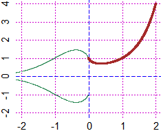 |
# It is easy to integrate numerically and graphically functions that are not easy to
# study "by hand". See here for an example.
# An example of integral that you can not study by hand:
F = function(x) sqrt(3*x-x^3); integral(F, 0,3/2)
# 1.720722
# Note 1. If the integral between -Inf and Inf is 0 check whether the integer between 0
# and Inf is finite too: if it does not happen it means that the integral diverges (0
# is output only for a formal simplification).
# Note 2. To integrate a function between a and b if it is not defined in a point c
# between a and b, make the sum of the integral between a and c and that between c and b.
#
# See here how to calculate areas using integrals
 # If F is a function of at least 2 variables, if two of these are u and v,
# derivxy(F,u,v) computes the second partial derivative with respect to u and v,
# derivyx(F,u,v) that with respect to v and u (xy and yx indicate that the derivatives
# are "crossed", even if the variables are not x and y). deriv2(F,u) computes the 2nd
# derivative respect to u.
# If F is a function of x and y, hessian(F,a,b) (see) computes the hessian of F in (a,b).
# (we remember that if in (x,y) all partial derivatives are zero and the hessian is
# negative/null/positive, then it is a saddle point / we cannot conlude anything /
# it is a min/max point if deriv2 respect to x is > / < 0 )
F = function(x,y,z) 5*x^2*y^3+x^3*z
deriv(F,"x"); deriv(F,"z")
# 5*(2*x)*y^3+3*x^2*z x^3
deriv2(F,"y"); deriv2(F,"z")
# 5*x^2*(3*(2*y)) 0
derivxy(F,"x","y"); derivxy(F,"x","z")
# 5*(2*x)*(3*y^2) 3*x^2
#
Q = function(x,y) x^4+6*x^2*y^2+y^4-32*(x^2+y^2)
# If F is a function of at least 2 variables, if two of these are u and v,
# derivxy(F,u,v) computes the second partial derivative with respect to u and v,
# derivyx(F,u,v) that with respect to v and u (xy and yx indicate that the derivatives
# are "crossed", even if the variables are not x and y). deriv2(F,u) computes the 2nd
# derivative respect to u.
# If F is a function of x and y, hessian(F,a,b) (see) computes the hessian of F in (a,b).
# (we remember that if in (x,y) all partial derivatives are zero and the hessian is
# negative/null/positive, then it is a saddle point / we cannot conlude anything /
# it is a min/max point if deriv2 respect to x is > / < 0 )
F = function(x,y,z) 5*x^2*y^3+x^3*z
deriv(F,"x"); deriv(F,"z")
# 5*(2*x)*y^3+3*x^2*z x^3
deriv2(F,"y"); deriv2(F,"z")
# 5*x^2*(3*(2*y)) 0
derivxy(F,"x","y"); derivxy(F,"x","z")
# 5*(2*x)*(3*y^2) 3*x^2
#
Q = function(x,y) x^4+6*x^2*y^2+y^4-32*(x^2+y^2)
 # deriv(Q,"x") and deriv(Q,"y") are 0 in (0,0).
# To calculate hessian the variables must be x and y
hessian(Q,0,0); hessian(Q,0,4); hessian(Q,2,-2)
# 4096 16384 -8192
deriv2(Q,"x")
# 4 * (3 * x^2) + 6 * 2 * y^2 - 32 * 2
# In (0,0) the hessian in > 0 and deriv2 respect to x is > 0: max point
# And indeed:
MAXF2(Q, -1,1, -1,1)
# 0 0 0 In (0,0) I have a max, and Q(0,0) = 0
#
# The gradient of Q, grad(Q), is x,y -> ( d(Q(x,y)/dx, d(Q(x,y)/dy ):
c( deriv(Q,"x"), deriv(Q,"y") )
# 4*x^3+12*x*y^2-64*x 12*x^2*y+4*y^3-64*y
# For the use of this concept see here.
#
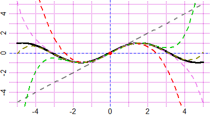
# For Taylor polynomials see here.
# deriv(Q,"x") and deriv(Q,"y") are 0 in (0,0).
# To calculate hessian the variables must be x and y
hessian(Q,0,0); hessian(Q,0,4); hessian(Q,2,-2)
# 4096 16384 -8192
deriv2(Q,"x")
# 4 * (3 * x^2) + 6 * 2 * y^2 - 32 * 2
# In (0,0) the hessian in > 0 and deriv2 respect to x is > 0: max point
# And indeed:
MAXF2(Q, -1,1, -1,1)
# 0 0 0 In (0,0) I have a max, and Q(0,0) = 0
#
# The gradient of Q, grad(Q), is x,y -> ( d(Q(x,y)/dx, d(Q(x,y)/dy ):
c( deriv(Q,"x"), deriv(Q,"y") )
# 4*x^3+12*x*y^2-64*x 12*x^2*y+4*y^3-64*y
# For the use of this concept see here.
#
# For Taylor polynomials see here.
 #
# For integrals of the functions of two variables we can use the command INTEGRAL. See here.
#
# For integrals of the functions of two variables we can use the command INTEGRAL. See here.
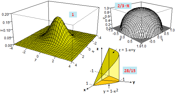 # For volumes of solids of revolution see here.
 # For max and min of functions of two variables see here (commands MINF2, MAXF2).
#
# The mean value (not of a set of values but) of a variable quantity depends on
# which variable one wants to make it dependent on.
# If f is a continuous positive function on [a,b] we assume as mean of f on [a,b] the
# value m such that the area of the drawn rectangle equals the result of integrating f
# on [a,b]: m = integral(f, a,b) / (b-a)
# For max and min of functions of two variables see here (commands MINF2, MAXF2).
#
# The mean value (not of a set of values but) of a variable quantity depends on
# which variable one wants to make it dependent on.
# If f is a continuous positive function on [a,b] we assume as mean of f on [a,b] the
# value m such that the area of the drawn rectangle equals the result of integrating f
# on [a,b]: m = integral(f, a,b) / (b-a)
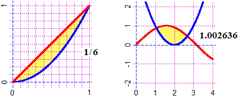
 # For example, the problem:
# Calculate the average value of the chord of a semi-circle
# (of radius 1) that is parallel to the diameter
# depends on whether, for example, we identify the position of the chord using
# L, D or A. I can obtain 1, π/2 or 4/π.
# For example, the problem:
# Calculate the average value of the chord of a semi-circle
# (of radius 1) that is parallel to the diameter
# depends on whether, for example, we identify the position of the chord using
# L, D or A. I can obtain 1, π/2 or 4/π.
 FL = function(x) x; I = integral(FL, 0,2) / 2; I
# 1
FD = function(x) 2*sqrt(1-x^2); I = integral(FD, 0,1)/1; I
# 1.570796
pi/2
# 1.570796
FA = function(t) 2*sin(t); I = integral(FA, 0,pi/2) / (pi/2); I
# 1.27324
I*pi
# 4
Other examples of use
FL = function(x) x; I = integral(FL, 0,2) / 2; I
# 1
FD = function(x) 2*sqrt(1-x^2); I = integral(FD, 0,1)/1; I
# 1.570796
pi/2
# 1.570796
FA = function(t) 2*sin(t); I = integral(FA, 0,pi/2) / (pi/2); I
# 1.27324
I*pi
# 4
Other examples of use