source("http://macosa.dima.unige.it/r.R") # If I have not already loaded the library
---------- ---------- ---------- ---------- ---------- ---------- ---------- ----------
S 12 Regression. Splines. Curve fitting. Moving average (or mean).
Linear, quadratic and cubic regression: the linear function with graph for a given
point (p,q) and the generic linear, quadratic and cubic functions that "best"
approximate some experimental data (x,y). Commands:
regression(x,y,p,q), regression1(x,y), regression2(x,y), regression3(x,y)
If the points are 2, 3 or 4 regression1, regression2 and regression3 find exactly the
curve. In these cases we have an interpolation.
We also see how splines (approximating function graphs or curves) can be calculated
(typical instrument to obtain a smooth curve in agreement with a finite number of
digital information). Also the splines are examples of interpolation.
For a more complete method of studyng linear regression (and the command LR) see here.
If the "x" are too large [for example x=c(2007,2012,…)] an error message may appear.
In this case you can modify x (x-2000) and find the regression rB (of x-2000), and
then modify it [take r(x) = rB(x-2000)]
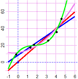
x = c(-0.2, 1.3, 1.7, 3.2, 4.1, 4.6)
y = c(9.1, 17.5, 20.7, 25.4, 35.7, 51.2)
Plane(-1,6,-10,70); POINT(x,y,1)
regression(x,y, 0,0); POINT(0,0,"blue")
# 9.829 * x
f = function(x) 9.829 * x; graph(f,-1,6, "red")
regression1(x,y)
# 7.628 * x + 7.911
g = function(x) 7.628 * x + 7.911; graph(g,-1,6, "blue")
regression2(x,y)
# 1.37 * x^2 + 1.38 * x + 11.2
h = function(x) 1.37 * x^2 + 1.38 * x + 11.2; graph(h,-1,6, "violet")
regression3(x,y)
# 1.21 * x^3 + -6.3 * x^2 + 11.9 * x + 11.6
k = function(x) 1.21 * x^3 + -6.3 * x^2 + 11.9 * x + 11.6; graph(k,-1,6, "green")
POINT(0,0,"blue"); POINT(x,y,1)
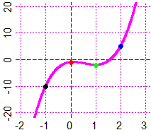 # On the right, the curve that goes exactly for (-1,-10),(0,-1),(1,-2),(2,5)
Plane(-2,3,-20,20)
POINT(-1,-10, 1); POINT(0,-1,"red"); POINT(1,-2,"green"); POINT(2,5,"blue")
regression3( c(-1,0,1,2), c(-10,-1,-2,5) )
# 3 * x^3 + -5 * x^2 + 1 * x + -1
f = function(x) 3 * x^3 + -5 * x^2 + 1 * x + -1
graph(f,-2,3, 6)
POINT(-1,-10, 1); POINT(0,-1,"red"); POINT(1,-2,"green"); POINT(2,5,"blue")
# It is the same function that we obtain with xy_4(c(-1,0,1,2), c(-10,-1,-2,5)) [see]
# The cubic spline that interpolates the points x,y (see):
# On the right, the curve that goes exactly for (-1,-10),(0,-1),(1,-2),(2,5)
Plane(-2,3,-20,20)
POINT(-1,-10, 1); POINT(0,-1,"red"); POINT(1,-2,"green"); POINT(2,5,"blue")
regression3( c(-1,0,1,2), c(-10,-1,-2,5) )
# 3 * x^3 + -5 * x^2 + 1 * x + -1
f = function(x) 3 * x^3 + -5 * x^2 + 1 * x + -1
graph(f,-2,3, 6)
POINT(-1,-10, 1); POINT(0,-1,"red"); POINT(1,-2,"green"); POINT(2,5,"blue")
# It is the same function that we obtain with xy_4(c(-1,0,1,2), c(-10,-1,-2,5)) [see]
# The cubic spline that interpolates the points x,y (see):
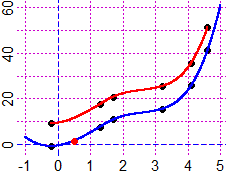
 x = c(-0.2, 1.3, 1.7, 3.2, 4.1, 4.6)
y = c(9.1, 17.5, 20.7, 25.4, 35.7, 51.2)
BF=3; HF=2.5; Plane(-1,5,-5,65); POINT(x,y,1)
SF = splinefun(x,y); graph2(SF,-0.2,4.6, "red")
POINT(x,y-10,1); SF1=splinefun(x,y-10); graph2(SF1,-1,5,"blue")
# The "extended" (blue) curve that passes by the same points, lowered by 10 (the inter-
# polation used to find the curve outside the known points is called extrapolation)
# Obviously if I want to find a value of y I can use splinefun(x,y). For example:
splinefun(x,y-10)(0.5) # or: SF1(0.5)
# 1.383585
POINT(0.5, splinefun(x,y-10)(0.5), "red")
# splinefunD(…, …, N, col) plots the graph of the Nth derivative:
BF=4.5; HF=3; Plane(-1,5, -30,65)
graph2(SF,-1,5, "red"); POINT(x,y,1)
splinefunD(x,y,1,"blue"); splinefunD(x,y,2,"seagreen"); splinefunD(x,y,3,"orange")
text(3.8,5,"D1"); text(2.7,-5,"D2"); text(0.5,-14,"D3")
x = c(-0.2, 1.3, 1.7, 3.2, 4.1, 4.6)
y = c(9.1, 17.5, 20.7, 25.4, 35.7, 51.2)
BF=3; HF=2.5; Plane(-1,5,-5,65); POINT(x,y,1)
SF = splinefun(x,y); graph2(SF,-0.2,4.6, "red")
POINT(x,y-10,1); SF1=splinefun(x,y-10); graph2(SF1,-1,5,"blue")
# The "extended" (blue) curve that passes by the same points, lowered by 10 (the inter-
# polation used to find the curve outside the known points is called extrapolation)
# Obviously if I want to find a value of y I can use splinefun(x,y). For example:
splinefun(x,y-10)(0.5) # or: SF1(0.5)
# 1.383585
POINT(0.5, splinefun(x,y-10)(0.5), "red")
# splinefunD(…, …, N, col) plots the graph of the Nth derivative:
BF=4.5; HF=3; Plane(-1,5, -30,65)
graph2(SF,-1,5, "red"); POINT(x,y,1)
splinefunD(x,y,1,"blue"); splinefunD(x,y,2,"seagreen"); splinefunD(x,y,3,"orange")
text(3.8,5,"D1"); text(2.7,-5,"D2"); text(0.5,-14,"D3")
 # D1, D2, D3: branches of parabolas, straight lines, horizontal lines.
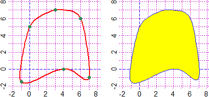
# If you have some points of a closed curve you can approximate it with the command
# splineC(x,y,ColBorder,ColInside), or splinC if you want a thin-stroke curve. If you
# choose NULL as internal color the figure is transparent.
BF=3; HF=3; PLANE(-2,8, -2,8)
u=c( -1, 4, 7,6,3,0)
v=c(-1.5,0,-1,6,7,5)
splineC(u,v,"red",NULL); POINT(u,v,"seagreen")
PLANE(-2,8, -2,8); splinC(u,v,"blue","yellow")
# D1, D2, D3: branches of parabolas, straight lines, horizontal lines.
# If you have some points of a closed curve you can approximate it with the command
# splineC(x,y,ColBorder,ColInside), or splinC if you want a thin-stroke curve. If you
# choose NULL as internal color the figure is transparent.
BF=3; HF=3; PLANE(-2,8, -2,8)
u=c( -1, 4, 7,6,3,0)
v=c(-1.5,0,-1,6,7,5)
splineC(u,v,"red",NULL); POINT(u,v,"seagreen")
PLANE(-2,8, -2,8); splinC(u,v,"blue","yellow")
 # The points used to trace the curve are in splineCx(x,y) and splineCy(x,y)
length(splineCx(u,v))
# 104
c( splineCx(u,v)[1],splineCy(u,v)[1] )
# -1.0 -1.5
c( splineCx(u,v)[2],splineCy(u,v)[2] )
# -0.8442124 -1.6377163
# If you want to have approximately the area of the closed curve you can use areaPol:
areaPol(splineCx(u,v),splineCy(u,v))
# 53.88609
# splineL(x,y,ColBorder), and splinL, do not close the curve.
# The points used to trace the curve are in splineCx(x,y) and splineCy(x,y)
length(splineCx(u,v))
# 104
c( splineCx(u,v)[1],splineCy(u,v)[1] )
# -1.0 -1.5
c( splineCx(u,v)[2],splineCy(u,v)[2] )
# -0.8442124 -1.6377163
# If you want to have approximately the area of the closed curve you can use areaPol:
areaPol(splineCx(u,v),splineCy(u,v))
# 53.88609
# splineL(x,y,ColBorder), and splinL, do not close the curve.
 BF=1.8; HF=BF*340/270
BOXW(0,270,0,340)
x=c(22,34,38, 35, 7, 2, 15, 52,114,194,221,233,231,228,227,243,259,
255,233,239,235,238,229,226,236,217,201,154,157)
y=c( 4,55,92,129,187,224,278,315,331,307,271,230,216,211,205,174.5,144,
131,130,119,113,109,102, 92, 68, 59, 55, 57, 4)
splineL(x,y,"pink"); splinL(x,y,"brown")
#
Point(x,y, "red"); gridVC(seq(0,270,50),"blue"); gridHC(seq(0,340,50),"blue")
# If we want to approximate points with a curve y = A·exp(B·x) we can use regression1
# after transforming y-coordinates by the logarithmic function. If we want approximate
# them with a polynomial curve we can transform x-coordinates too: see here
BF=1.8; HF=BF*340/270
BOXW(0,270,0,340)
x=c(22,34,38, 35, 7, 2, 15, 52,114,194,221,233,231,228,227,243,259,
255,233,239,235,238,229,226,236,217,201,154,157)
y=c( 4,55,92,129,187,224,278,315,331,307,271,230,216,211,205,174.5,144,
131,130,119,113,109,102, 92, 68, 59, 55, 57, 4)
splineL(x,y,"pink"); splinL(x,y,"brown")
#
Point(x,y, "red"); gridVC(seq(0,270,50),"blue"); gridHC(seq(0,340,50),"blue")
# If we want to approximate points with a curve y = A·exp(B·x) we can use regression1
# after transforming y-coordinates by the logarithmic function. If we want approximate
# them with a polynomial curve we can transform x-coordinates too: see here

 #
# See here to see other methods of curve fitting (with the commands F_RUN1, F_RUN2,
# ... F_RUN6).
#
# See here to see other methods of curve fitting (with the commands F_RUN1, F_RUN2,
# ... F_RUN6).

 #
# An example of use of regression.
#
# An example of use of regression.
# A ball is allowed to fall freely under gravity. The image on the
# right was captured with a stroboscopic flash at 30 flashes per
# second. I look for the curve y=c2*x^2+c1*x+c0 that passes through
# the points and I take g = 2*c2 (s = s0+v0*t+a/2*t^2, a = g; the first
# flash does not correspond exactly to the release of the ball; so the
# low is not s = a/2*t^2).  How much is g?
# The distance (in meters) of the ball from the initial position is
# approximately:
k = c(0,0.03,0.06,0.09,0.14,0.20,0.27,0.35,0.44,
    0.55,0.67,0.80,0.94,1.08,1.24,1.41,1.60,1.77)
length(k)
# 18                     number of distances
t = 1/30*(0:17)        # the times (in seconds)
regression2(t,k)       # the regression of 2nd order
# 4.92 * x^2 + 0.345 * x + 0.00675
# I can take 2*4.9 = 9.8 as an approximation of g. |  |
#
# In this case I does not have a "fixed point" (1st flash does not correspond exactly
# to the release of the ball).
# How to proceed for a regression of the second order when I have a fixed point?
# Without using specific methods, I can do the following:
x = c(-0.2, 1.3, 1.7, 3.2, 4.1, 4.6)
y = c(9.1, 17.5, 20.7, 25.4, 35.7, 51.2)
Plane(-1,6,-10,70); POINT(x,y,"black")
# Without a fixed point:
regression2(x,y)
# 1.37 * x^2 + 1.38 * x + 11.2
h = function(x) 1.37*x^2 + 1.38*x + 11.2; graph2(h,-1,6, "magenta")
 # If I have the fixed point (3.2,25.4) I can force the passage for a large amount of
# points (for example 1e6) that are equal to (3.2,25.4)!
x1=c(rep(3.2,1e6),x); y1=c(rep(25.4,1e6),y)
Plane(-1,6,-10,70); POINT(x,y,"black")
regression2(x1,y1)
# 2.19 * x^2 + -2.91 * x + 12.3
h1 = function(x) 2.19 * x^2 + -2.91 * x + 12.3
graph2(h1,-1,6, "blue"); POINT(3.2,25.4, "red")
#
# Another example of use of regression:
# A car (initially) goes at a steady speed. The driver sees an obstacle and (after 1.5
# seconds) starts braking. Here are the photos taken every half second from the instant
# in which he saw the obstacle. What was the initial speed of the car?
# If I have the fixed point (3.2,25.4) I can force the passage for a large amount of
# points (for example 1e6) that are equal to (3.2,25.4)!
x1=c(rep(3.2,1e6),x); y1=c(rep(25.4,1e6),y)
Plane(-1,6,-10,70); POINT(x,y,"black")
regression2(x1,y1)
# 2.19 * x^2 + -2.91 * x + 12.3
h1 = function(x) 2.19 * x^2 + -2.91 * x + 12.3
graph2(h1,-1,6, "blue"); POINT(3.2,25.4, "red")
#
# Another example of use of regression:
# A car (initially) goes at a steady speed. The driver sees an obstacle and (after 1.5
# seconds) starts braking. Here are the photos taken every half second from the instant
# in which he saw the obstacle. What was the initial speed of the car?
 # Times (in seconds) and spaces (in meters):
s0 = c(1.5,2.0,2.5,3.0,3.5,4.0,4.5,5.0,5.5,6.0,6.5,7.0,7.5,8.0,8.5,9.0,9.5)
m0 = c( 70, 92,114,133,151,168,183,198,209,221,230,238,244,250,253,255,257)
# Since he has begun to brake:
s = s0-1.5; m = m0-70; s; m
# 0.0 0.5 1.0 1.5 2.0 2.5 3.0 3.5 4.0 4.5 5.0 5.5 6.0 6.5 7.0 7.5 8.0
# 0 22 44 63 81 98 113 128 139 151 160 168 174 180 183 185 187
# The graph (time,space):
Plane(-1/2,8.5, -1,190); POINT(s,m, "blue")
abovex("sec"); abovey("m")
# Times (in seconds) and spaces (in meters):
s0 = c(1.5,2.0,2.5,3.0,3.5,4.0,4.5,5.0,5.5,6.0,6.5,7.0,7.5,8.0,8.5,9.0,9.5)
m0 = c( 70, 92,114,133,151,168,183,198,209,221,230,238,244,250,253,255,257)
# Since he has begun to brake:
s = s0-1.5; m = m0-70; s; m
# 0.0 0.5 1.0 1.5 2.0 2.5 3.0 3.5 4.0 4.5 5.0 5.5 6.0 6.5 7.0 7.5 8.0
# 0 22 44 63 81 98 113 128 139 151 160 168 174 180 183 185 187
# The graph (time,space):
Plane(-1/2,8.5, -1,190); POINT(s,m, "blue")
abovex("sec"); abovey("m")
 # I want to impose that s(0)=0. I proceed as in the last example:
s1 = c(rep(0,1e6), s); m1 = c(rep(0,1e6), m)
regression2(s1,m1)
# -2.89 * x^2 + 46.5 * x + -2.89e-07 # I neglect -2.89e-07
F = function(x) -2.89 * x^2 + 46.5 * x
graph2(F,0,8, "brown") # See the chart above
# I find the derivative (I can find it "by hand" but ...)
deriv(F,"x")
# 46.5 - 2.89 * (2 * x)
# The initial speed is 46.5 m/s.
46.5/1000*60*60
# 167.4 167 km/h
# It is easy to calculate the moving average (or moving mean) of a data sequence (to
# smooth out the fluctuations). An example:
# I have the file of "mm of monthly rainfall in Genoa in the period 1984-92", here.
# In Windows, I can load the file or I can copy the file to the clipboard and then with
readLines("clipboard")
# if I want, I can view the file:
# [1] "# mm of monthly rainfall in Genoa in the period 1984-92; make the moving averages"
# [2] "1,41"
# ...
# [109] "108,72"
# In any case, I put the table in a variable (I use the same separator ","; I have no line to jump)
rain = read.table("clipboard",sep=",")
# In Mac I can't load a table with "clipboard". I can copy the file in a text-file and use this;
# here I copied it in "macosa.dima.unige.it/R/rain.txt"; in the same way I proceed if I copied
# it to my PC. Obviously I can proceed like this even in Windows.
readLines("http://macosa.dima.unige.it/R/rain.txt") # if I want to see the file
rain = read.table("http://macosa.dima.unige.it/R/rain.txt",sep=",")
# If I want I can view (better) the file:
str(rain)
# 'data.frame': 108 obs. of 2 variables:
# $ V1: int 1 2 3 4 5 6 7 8 9 10 ...
# $ V2: int 41 44 72 79 197 62 0 200 52 95 ...
# I obtain the first graph with:
x = rain$V1; y = rain$V2; max(y)
# 423
BF=6; HF=2
Plane(0,110,0,450)
polylin(x,y, "red")
Point(x,y, "blue")
# I want to impose that s(0)=0. I proceed as in the last example:
s1 = c(rep(0,1e6), s); m1 = c(rep(0,1e6), m)
regression2(s1,m1)
# -2.89 * x^2 + 46.5 * x + -2.89e-07 # I neglect -2.89e-07
F = function(x) -2.89 * x^2 + 46.5 * x
graph2(F,0,8, "brown") # See the chart above
# I find the derivative (I can find it "by hand" but ...)
deriv(F,"x")
# 46.5 - 2.89 * (2 * x)
# The initial speed is 46.5 m/s.
46.5/1000*60*60
# 167.4 167 km/h
# It is easy to calculate the moving average (or moving mean) of a data sequence (to
# smooth out the fluctuations). An example:
# I have the file of "mm of monthly rainfall in Genoa in the period 1984-92", here.
# In Windows, I can load the file or I can copy the file to the clipboard and then with
readLines("clipboard")
# if I want, I can view the file:
# [1] "# mm of monthly rainfall in Genoa in the period 1984-92; make the moving averages"
# [2] "1,41"
# ...
# [109] "108,72"
# In any case, I put the table in a variable (I use the same separator ","; I have no line to jump)
rain = read.table("clipboard",sep=",")
# In Mac I can't load a table with "clipboard". I can copy the file in a text-file and use this;
# here I copied it in "macosa.dima.unige.it/R/rain.txt"; in the same way I proceed if I copied
# it to my PC. Obviously I can proceed like this even in Windows.
readLines("http://macosa.dima.unige.it/R/rain.txt") # if I want to see the file
rain = read.table("http://macosa.dima.unige.it/R/rain.txt",sep=",")
# If I want I can view (better) the file:
str(rain)
# 'data.frame': 108 obs. of 2 variables:
# $ V1: int 1 2 3 4 5 6 7 8 9 10 ...
# $ V2: int 41 44 72 79 197 62 0 200 52 95 ...
# I obtain the first graph with:
x = rain$V1; y = rain$V2; max(y)
# 423
BF=6; HF=2
Plane(0,110,0,450)
polylin(x,y, "red")
Point(x,y, "blue")
 # To put in D2 the moving averages (of order 3) of D1[1], ..., D2[nD] I can use:
# D2 = D1[1]; for ( i in 2:(nD-1) ) D2[i] = (D1[i-1]+D1[i]+D1[i+1])/3; D2 = c(D2,D1[nD])
# How to obtain the second graph:
n = 108
D1 = y; nD = n
D2 = D1[1]; for ( i in 2:(nD-1) ) D2[i] = (D1[i-1]+D1[i]+D1[i+1])/3; D2 = c(D2,D1[nD])
y1=D2
max(y1)
# 230
Plane(0,110,0,250)
polylin(x,y1,"red"); Point(x,y1,"blue")
#
# For the last graph I make the moving averages 4 times:
D1 = y; nD = n
for(i in 1:4) {
D2 = D1[1]; for ( i in 2:(nD-1) ) D2[i] = (D1[i-1]+D1[i]+D1[i+1])/3; D2 = c(D2,D1[nD])
D1=D2}
y2=D2
max(y2)
# 170.2099
Plane(0,110,0,200)
polylin(x,y2,"red")
# I mark the division into years:
for(i in 0:10) segm(1+i*12,0, 1+i*12,200, 0)
#
# Another example of "moving mean":
# the human growth curve, from age two through adulthood
# (height velocity, 35 males, 1980)
a=c(2.0,2.4,2.9,3.5,4.0,4.5,5,5.4,6.0,6.5,7.0,7.4,8.0,8.5,9.0,9.4,9.7,10.6,11.6,
11.9,12.4,13.0,13.4,13.8,14.0,14.3,14.8,14.9,15.5,15.9,15.9,16.5,17.0,17.2,17.4)
v=c(11.6,8.8,7.6,6.4,8.4,6.5,6,6.1,7.6,6.5,6.3,6.5,5.4,6.3,5.2,4.9,4.8,2.9,7.6,
6.8,5.5,5.5,7.6,10.3,9.9,12,10.4,8.3,5.1,5.3,5.2,4.4,3.7,3.9,2.0)
BF=6; HF=3.5
Plane(0,20, 0,13)
abovex("age (years)"); abovey("growth velocity (cm/year)")
POINT(a,r, "brown")
n = length(a)
D1 = v; nD = n
for(i in 1:4) {
D2 = D1[1]; for ( i in 2:(nD-1) ) D2[i] = (D1[i-1]+D1[i]+D1[i+1])/3; D2 = c(D2,D1[nD])
D1=D2}
v1=D2
polylin(a,v1,"seagreen")
# To put in D2 the moving averages (of order 3) of D1[1], ..., D2[nD] I can use:
# D2 = D1[1]; for ( i in 2:(nD-1) ) D2[i] = (D1[i-1]+D1[i]+D1[i+1])/3; D2 = c(D2,D1[nD])
# How to obtain the second graph:
n = 108
D1 = y; nD = n
D2 = D1[1]; for ( i in 2:(nD-1) ) D2[i] = (D1[i-1]+D1[i]+D1[i+1])/3; D2 = c(D2,D1[nD])
y1=D2
max(y1)
# 230
Plane(0,110,0,250)
polylin(x,y1,"red"); Point(x,y1,"blue")
#
# For the last graph I make the moving averages 4 times:
D1 = y; nD = n
for(i in 1:4) {
D2 = D1[1]; for ( i in 2:(nD-1) ) D2[i] = (D1[i-1]+D1[i]+D1[i+1])/3; D2 = c(D2,D1[nD])
D1=D2}
y2=D2
max(y2)
# 170.2099
Plane(0,110,0,200)
polylin(x,y2,"red")
# I mark the division into years:
for(i in 0:10) segm(1+i*12,0, 1+i*12,200, 0)
#
# Another example of "moving mean":
# the human growth curve, from age two through adulthood
# (height velocity, 35 males, 1980)
a=c(2.0,2.4,2.9,3.5,4.0,4.5,5,5.4,6.0,6.5,7.0,7.4,8.0,8.5,9.0,9.4,9.7,10.6,11.6,
11.9,12.4,13.0,13.4,13.8,14.0,14.3,14.8,14.9,15.5,15.9,15.9,16.5,17.0,17.2,17.4)
v=c(11.6,8.8,7.6,6.4,8.4,6.5,6,6.1,7.6,6.5,6.3,6.5,5.4,6.3,5.2,4.9,4.8,2.9,7.6,
6.8,5.5,5.5,7.6,10.3,9.9,12,10.4,8.3,5.1,5.3,5.2,4.4,3.7,3.9,2.0)
BF=6; HF=3.5
Plane(0,20, 0,13)
abovex("age (years)"); abovey("growth velocity (cm/year)")
POINT(a,r, "brown")
n = length(a)
D1 = v; nD = n
for(i in 1:4) {
D2 = D1[1]; for ( i in 2:(nD-1) ) D2[i] = (D1[i-1]+D1[i]+D1[i+1])/3; D2 = c(D2,D1[nD])
D1=D2}
v1=D2
polylin(a,v1,"seagreen")
 Other examples of use