
source("http://macosa.dima.unige.it/r.R")    # If I have not already loaded the library
---------- ---------- ---------- ---------- ---------- ---------- ---------- ----------
S 18 Animations
While clock() and clock2(12,25,40) display the current time or hour that is written, Hour(), Minute() and Second() contain numerical information about the current time. Sec() provides the number of seconds since the start of the program; wait(x) does spend x seconds (useful commands for animations). |  |
These commands can be used to create animations.
If I want, I can store them in file that I can
load with source command.
For an example run the line:
source("http://macosa.dima.unige.it/R/pythag.txt")
or:
source("http://macosa.dima.unige.it/R/pitag.txt")
( use:  http://macosa.dima.unige.it/R/pitag.txt
  in the browser if you want see the file )

For another example see here |
 |
 We have already seen animations here.
I can also store individual images and then merge them into an animated gif (see)
We have already seen animations here.
I can also store individual images and then merge them into an animated gif (see)
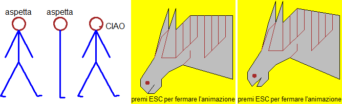 # Program that produces the pictures here above, on the left:
HF=3; BF=3
boxW(0,100,0,100)
for(k in 0:10) {
BoxW(0,100, 0,100)
circle(50,82, 7, "brown"); text(50,95,"aspetta")
polyline( c(55,50,50),
c(0,0,75), "blue" );
wait(0.6); BoxW(0,100, 0,100)
circle(50,82, 7, "brown"); text(50,95,"aspetta")
polyline( c(35,30,50,70,75,70,50,50,35,50,65),
c(1.5,2,40,2,2.5, 2,40,75,45,75,45), "blue" );
wait(0.8) }
polyline(c(53.5,55.85),c(79,79), "brown"); text(71,80,"CIAO"); CLEAN(0,100, 90,100)
# CLEAN overlaps a white rectangle
BOX() # <- to overlay a grid, use one of these 3
BOXw() # commands (usual, without axes, great axes)
BOXg() # For the horse see here.
# Program that produces the pictures here above, on the left:
HF=3; BF=3
boxW(0,100,0,100)
for(k in 0:10) {
BoxW(0,100, 0,100)
circle(50,82, 7, "brown"); text(50,95,"aspetta")
polyline( c(55,50,50),
c(0,0,75), "blue" );
wait(0.6); BoxW(0,100, 0,100)
circle(50,82, 7, "brown"); text(50,95,"aspetta")
polyline( c(35,30,50,70,75,70,50,50,35,50,65),
c(1.5,2,40,2,2.5, 2,40,75,45,75,45), "blue" );
wait(0.8) }
polyline(c(53.5,55.85),c(79,79), "brown"); text(71,80,"CIAO"); CLEAN(0,100, 90,100)
# CLEAN overlaps a white rectangle
BOX() # <- to overlay a grid, use one of these 3
BOXw() # commands (usual, without axes, great axes)
BOXg() # For the horse see here.
 # Run the following three lines ...
f = function(x) ifelse(x != 0, cos(1/x)*x, 0); BF=4; HF=3; a = 4
for(i in 1:8) {a=a/2; graph2F(f,-a,a,"blue"); if(a<2) abovex("I made a zoom"); wait(3)}
underx("STOP") # see
# Run the following three lines ...
f = function(x) ifelse(x != 0, cos(1/x)*x, 0); BF=4; HF=3; a = 4
for(i in 1:8) {a=a/2; graph2F(f,-a,a,"blue"); if(a<2) abovex("I made a zoom"); wait(3)}
underx("STOP") # see
BF=4; HF=4
PLANE(-3,3, -3,3)
q=1; POINT(q,0, "red"); line2p(-1,-2, -1,2, "red")
parabola <- function(x,y) y^2-4*q*x
CURVE(parabola, "black")
fig <- recordPlot()
# the superior part of the parabola
f = function(x) sqrt(4*q*x)
for(x in (22:0)/10) {wait(0.3);replayPlot(fig)
POINT(q,0, "red"); line2p(-1,-2, -1,2, "red")
CURVE(parabola, "black")
y = f(x); POINT(x,y, "brown")
polyL( c(-1,x,1), c(y,y,0), "brown")}
# a moment of the animation -> |  |
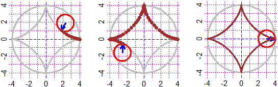
 # The construction of an asteroid (the figure drawn by a point of a circle that
# rotates on a larger circle)
PLANE(-4,4, -4,4)
f <- function(t) 4*cos(t)^3; g <- function(t) 4*sin(t)^3
circle(0,0, 4, "grey"); param(f,g, 0,2*pi, "grey"); fig0 <- fig <- recordPlot()
i <- 0; x <- 4; y <- 0; dt <- 0.3
while(i < 90) {replayPlot(fig); POINT(x,y,"brown"); fig <- recordPlot()
i <- i+1
t <- 2*pi/90*i; circle(3*cos(t),3*sin(t), 1, "red");
arrow(3*cos(t),3*sin(t), 4*cos(t)^3, 4*sin(t)^3, "blue");
x <- c(x,4*cos(t)^3); y <- c(y,4*sin(t)^3); wait(dt) }
wait(dt); replayPlot(fig0); param(f,g, 0,2*pi, "brown")
# For a version without grid click.
# The construction of an asteroid (the figure drawn by a point of a circle that
# rotates on a larger circle)
PLANE(-4,4, -4,4)
f <- function(t) 4*cos(t)^3; g <- function(t) 4*sin(t)^3
circle(0,0, 4, "grey"); param(f,g, 0,2*pi, "grey"); fig0 <- fig <- recordPlot()
i <- 0; x <- 4; y <- 0; dt <- 0.3
while(i < 90) {replayPlot(fig); POINT(x,y,"brown"); fig <- recordPlot()
i <- i+1
t <- 2*pi/90*i; circle(3*cos(t),3*sin(t), 1, "red");
arrow(3*cos(t),3*sin(t), 4*cos(t)^3, 4*sin(t)^3, "blue");
x <- c(x,4*cos(t)^3); y <- c(y,4*sin(t)^3); wait(dt) }
wait(dt); replayPlot(fig0); param(f,g, 0,2*pi, "brown")
# For a version without grid click.
 # Another example here.
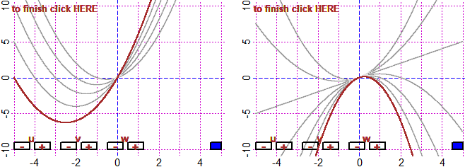
 # On the construction of curves with parameters we have already focused in S01.
# Here we see how to make them animated.
# I have to use u (v, w, k) as parameters and du (dv, dw, dk) as steps.
# The commands are fun1P, …, fun4P. By clicking I can change the parameters.
# The previous curve is drawn in gray.
# Click the blue button to see the charts thicker.
BF=3.5; HF=3.5 # If you want you can increase the size
F = function(x) 1+u*x
u=1; du=1; fun1P(F, -5,5, -5,5)
# On the construction of curves with parameters we have already focused in S01.
# Here we see how to make them animated.
# I have to use u (v, w, k) as parameters and du (dv, dw, dk) as steps.
# The commands are fun1P, …, fun4P. By clicking I can change the parameters.
# The previous curve is drawn in gray.
# Click the blue button to see the charts thicker.
BF=3.5; HF=3.5 # If you want you can increase the size
F = function(x) 1+u*x
u=1; du=1; fun1P(F, -5,5, -5,5)

 BF=3.5; HF=3.5 # If you want you can increase the size
G = function(x) v+u*x
u=1; du=1; v=1; dv=0.5; fun2P(G, -5,5, -5,5)
BF=3.5; HF=3.5 # If you want you can increase the size
G = function(x) v+u*x
u=1; du=1; v=1; dv=0.5; fun2P(G, -5,5, -5,5)

 BF=5; HF=4; H = function(x) u*x^2+v*x+w
u=1; du=0.5; v=1; dv=1; w=0; dw=0.5; fun3P(H,-5,5, -10,10)
BF=5; HF=4; H = function(x) u*x^2+v*x+w
u=1; du=0.5; v=1; dv=1; w=0; dw=0.5; fun3P(H,-5,5, -10,10)
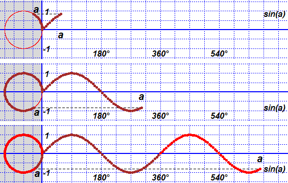
 BF=8; HF=4
M = function(x) w*sin(x*u)+k*sin(x*v)
u=1; du=0.5; v=1; dv=0.5; w=1; dw=0.5; k=1; dk=0.5; fun4P(M,-10,50, -4,4)
BF=8; HF=4
M = function(x) w*sin(x*u)+k*sin(x*v)
u=1; du=0.5; v=1; dv=0.5; w=1; dw=0.5; k=1; dk=0.5; fun4P(M,-10,50, -4,4)
 # But if the ratio between the two periods is not rational the sum is not periodic
u=1; du=sqrt(1/2); v=1; dv=0.5; w=1; dw=0.5; k=1; dk=0.5; fun4P(M,-10,50, -4,4)
# But if the ratio between the two periods is not rational the sum is not periodic
u=1; du=sqrt(1/2); v=1; dv=0.5; w=1; dw=0.5; k=1; dk=0.5; fun4P(M,-10,50, -4,4)
 # If I want, I can use Family=1 to construct a family of curves
BF=5; HF=4; H = function(x) u*x^2+v*x+w
Family = 1
u=1; du=0.5; v=1; dv=1; w=0; dw=0.5; fun3P(H,-5,5, -10,10)
# On the left, if I click "+v". On the right, if I click "-u".
# If I want, I can use Family=1 to construct a family of curves
BF=5; HF=4; H = function(x) u*x^2+v*x+w
Family = 1
u=1; du=0.5; v=1; dv=1; w=0; dw=0.5; fun3P(H,-5,5, -10,10)
# On the left, if I click "+v". On the right, if I click "-u".
 # To return to the initial mode I can use Family=0
# If for some reason you want a monometric scale with Fun1P,…,Fun4P you must use HF/BF
# equale to (d-c)/(b-a) if (a,b) and (c,d) if the command is Fun…P(…,a,b, c,d). For
# example BF=4; HF=4 and Fun…P(…,-5,5, -5,5) or BF=6; HF=4 and Fun…P(…,-6,6, -4,4).
# Similarly we can use curve1P, …, curve4P
BF=3; HF=3; F = function(x,y) x^2+y^2-u
u = 2; du = 1/2; curve1P(F, -4,4, -4,4)
# To return to the initial mode I can use Family=0
# If for some reason you want a monometric scale with Fun1P,…,Fun4P you must use HF/BF
# equale to (d-c)/(b-a) if (a,b) and (c,d) if the command is Fun…P(…,a,b, c,d). For
# example BF=4; HF=4 and Fun…P(…,-5,5, -5,5) or BF=6; HF=4 and Fun…P(…,-6,6, -4,4).
# Similarly we can use curve1P, …, curve4P
BF=3; HF=3; F = function(x,y) x^2+y^2-u
u = 2; du = 1/2; curve1P(F, -4,4, -4,4)
 BF=5; HF=4; G <- function(x,y) x^2*u+y^2*v+w*x - k
u=2; du=1; v=2; dv=1; w=2; dw=1; k=2; dk=1; curve4P(G, -3,3, -3,3)
BF=5; HF=4; G <- function(x,y) x^2*u+y^2*v+w*x - k
u=2; du=1; v=2; dv=1; w=2; dw=1; k=2; dk=1; curve4P(G, -3,3, -3,3)
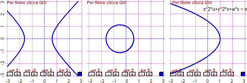 text(1.5,2.5,"x^2*u+y^2*v+w*x = k")
# I can then use polar1P, …, polar3P, with u (v, w) as parameters and du (dv, dw) as
# steps; polar…P uses automatically a monometric scale.
BF=3; HF=3; ro = function(teta) u*teta
u=1; du=0.5; polar1P(ro, 0,6*pi, -20,20, -20,20)
text(1.5,2.5,"x^2*u+y^2*v+w*x = k")
# I can then use polar1P, …, polar3P, with u (v, w) as parameters and du (dv, dw) as
# steps; polar…P uses automatically a monometric scale.
BF=3; HF=3; ro = function(teta) u*teta
u=1; du=0.5; polar1P(ro, 0,6*pi, -20,20, -20,20)
 # In the following example I use only 2 parameters
# The graph at the variation of t between 0 and 2π in (-3,9)×(-6,6)
ro <- function(t) u+v*cos(t)
u <- 2; du <- 0.1; v <- 2; dv <- 0.1; w <- 0; dw <- 0
BF=5; HF=4
polar3P(ro, 0,2*pi, -3,9, -6,6)
# In the following example I use only 2 parameters
# The graph at the variation of t between 0 and 2π in (-3,9)×(-6,6)
ro <- function(t) u+v*cos(t)
u <- 2; du <- 0.1; v <- 2; dv <- 0.1; w <- 0; dw <- 0
BF=5; HF=4
polar3P(ro, 0,2*pi, -3,9, -6,6)
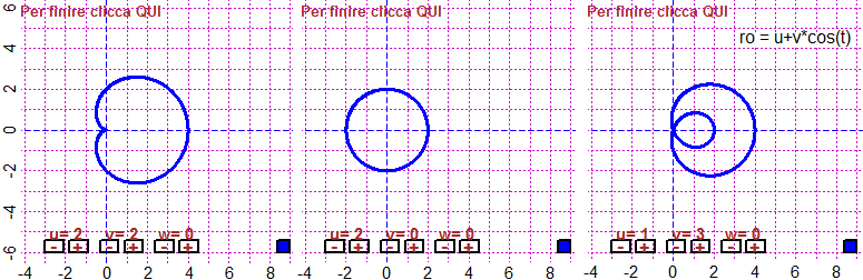 text(6,4.5,"ro = u+v*cos(t)")
# I can use "Family" with curve4P and polar3P, too.
Family=1
u <- 2; du <- 0.2; v <- 1/2; dv <- 1/2
polar3P(ro, 0,2*pi, -3,8, -5,5)
text(6,4.5,"ro = u+v*cos(t)")
# I can use "Family" with curve4P and polar3P, too.
Family=1
u <- 2; du <- 0.2; v <- 1/2; dv <- 1/2
polar3P(ro, 0,2*pi, -3,8, -5,5)
 c(u,v)
# 2.0 4.5
# v goes from 1/2 to 4.5 step 1/2
# Slope of a graph.
Define a function f (or g, h1, …). With the following command you get the graph of
f with input between a and b, output between c and d, with highlighted (x0,f(x0)).
If you click on a point, you have the graph of the line passing through the points of
the chart that have ascisse x0 and that of the point clicked. If you click the ascisse
x0 you have the tangent line. Press up to the left to finish.
Command: slope(f, a,b, c,d, x0)
Try with: h <- function(x) x^2; slope(h, -1,1.5, 0,3, 1)
This is a start to the concept of derivative
f <- function(x) cos(x)
slope(f, -3.2,0, -1.6,1.6, -pi/2)
#A dot is marked in the graph. By clicking near the graph, identify an
#abscissa. The line for P and the point of the graph with that abscissa
#are plotted. If you want, by clicking, you can repeat the test. When
#you want to stop click on top left. Now press ENTER. 1:
c(u,v)
# 2.0 4.5
# v goes from 1/2 to 4.5 step 1/2
# Slope of a graph.
Define a function f (or g, h1, …). With the following command you get the graph of
f with input between a and b, output between c and d, with highlighted (x0,f(x0)).
If you click on a point, you have the graph of the line passing through the points of
the chart that have ascisse x0 and that of the point clicked. If you click the ascisse
x0 you have the tangent line. Press up to the left to finish.
Command: slope(f, a,b, c,d, x0)
Try with: h <- function(x) x^2; slope(h, -1,1.5, 0,3, 1)
This is a start to the concept of derivative
f <- function(x) cos(x)
slope(f, -3.2,0, -1.6,1.6, -pi/2)
#A dot is marked in the graph. By clicking near the graph, identify an
#abscissa. The line for P and the point of the graph with that abscissa
#are plotted. If you want, by clicking, you can repeat the test. When
#you want to stop click on top left. Now press ENTER. 1:
 # See here for another specimen
 # See here for another specimen
 # See here for another specimen
 # See here for another specimen (the sum of two periodic f. can be not periodic)
 Other examples of use