source("http://macosa.dima.unige.it/r.R") # If I have not already loaded the library
---------- ---------- ---------- ---------- ---------- ---------- ---------- ----------
#
# Th symbol Inf represents the infinite. The "value" Inf is assumed when a number
# exceeds a certain value.
factorial(170); factorial(171)
# 7.257416e+306 Inf
# Similarly, the value 0 is assumed when the absolute value of a number is very small.
# For details:
.Machine
#
h = function(x) exp(-x)
Plane(0,10, -0,1); graph1(h, 0,10, "brown")
integral(h,0, Inf)
# 1
 # The limit of h as x -> Inf is 0:
h(1); h(10); h(100); h(Inf)
# 0.3678794 4.539993e-05 3.720076e-44 0
# Note: the limit of f(x) as x -> Inf can be estimated with f(Inf) not in all cases.
# It is good to evaluate f(x) as x grows to control. Ex .:
f = function(x) (1+1/x)^x; f(Inf)
# 1
# whereas the limit is e:
n = 1:8; f(10^n)
# 2.593742 2.704814 2.716924 2.718146 2.718268 2.718280 2.718282 2.718282
#
The limits of q(x) as q approaches 1 from the right and from the left can be different
q = function(x) (x^2-1)/(x^2-2*x+1); Plane(-2,2, -15,15); graph2(q,-2,2, "red")
# The limit of h as x -> Inf is 0:
h(1); h(10); h(100); h(Inf)
# 0.3678794 4.539993e-05 3.720076e-44 0
# Note: the limit of f(x) as x -> Inf can be estimated with f(Inf) not in all cases.
# It is good to evaluate f(x) as x grows to control. Ex .:
f = function(x) (1+1/x)^x; f(Inf)
# 1
# whereas the limit is e:
n = 1:8; f(10^n)
# 2.593742 2.704814 2.716924 2.718146 2.718268 2.718280 2.718282 2.718282
#
The limits of q(x) as q approaches 1 from the right and from the left can be different
q = function(x) (x^2-1)/(x^2-2*x+1); Plane(-2,2, -15,15); graph2(q,-2,2, "red")
 q(1-1E-2);q(1-1E-5);q(1-1E-10)
# -199 -199999 -Inf
q(1+1E-2);q(1+1E-5);q(1+1E-10)
# 201 200001 Inf
#
# There are sequences [ie functions F whose domain is the set 0,1,2,3,… or the set
# -2,-1,0,1,… or 6,7,8,9,…] such that F(n) can not be expressed with a simple term.
# Consider for example
# n√((n+1)·(n+2)·...·(n+n))/n for n = 1, 2, 3, …
# Let's see how to study the limit of F(n) as n that tends to infinity. First of all,
# I write the term in the easiest way to make calculations. In this particular case I
# have a product of terms that grow as both in value and quantity. I should rewrite
# F(n) as n√(n+1)·n√(n+2)·...·n√(n+n)/n
# I translate this into R, using a for loop to express the product of multiple terms:
F = function(n) {x=1; for(i in 1:n) x = x*(n+i)^(1/n); x/n}
# Study what's happening. Try with n power of 2. First I also try with n+1, to check
# that there are no differences if n is odd (with sequences, especially if there are
# some exponentiations, this can happen, even if I could understand that this is not
# the case).
n=2; c(F(n), F(n+1) )
# 1.732051 1.644141
n=2^2; c(F(n), F(n+1) )
# [1] 1.600543 1.574513
n=2^3; c(F(n), F(n+1) )
# [1] 1.535668 1.528503 All OK, remove F(n+1)
n=2^18; F(n)
# [1] 1.47152
n=2^19; F(n)
# [1] 1.471519
n=2^20; F(n)
# [1] 1.471518
n=2^21; F(n)
# [1] 1.471518
# I try with WolframAlpha if I can express this term more synthetically.
# I get 4/e. Verification:
4/exp(1)
# [1] 1.471518 OK!
# The study of a series: 1-1/2+1/3-1/4+1/5...
# The graph of N -> 1-1/2+ ... 1/N
a = function(n) (-1)^(n+1)/n # a(n): the nth element of the summation
N = function(n) seq(1,n,1) # N = 1 2 ... n
S = function(n) sum(a(N(n))) # sum a(1)+...a(n)
NMax = 20; Plane(0,NMax, 0,1)
for(i in 1:NMax) POINT(i,S(i), "brown")
for(i in 1:(NMax-1)) polyl(c(i,i+1),c(S(i),S(i+1)), "brown")
q(1-1E-2);q(1-1E-5);q(1-1E-10)
# -199 -199999 -Inf
q(1+1E-2);q(1+1E-5);q(1+1E-10)
# 201 200001 Inf
#
# There are sequences [ie functions F whose domain is the set 0,1,2,3,… or the set
# -2,-1,0,1,… or 6,7,8,9,…] such that F(n) can not be expressed with a simple term.
# Consider for example
# n√((n+1)·(n+2)·...·(n+n))/n for n = 1, 2, 3, …
# Let's see how to study the limit of F(n) as n that tends to infinity. First of all,
# I write the term in the easiest way to make calculations. In this particular case I
# have a product of terms that grow as both in value and quantity. I should rewrite
# F(n) as n√(n+1)·n√(n+2)·...·n√(n+n)/n
# I translate this into R, using a for loop to express the product of multiple terms:
F = function(n) {x=1; for(i in 1:n) x = x*(n+i)^(1/n); x/n}
# Study what's happening. Try with n power of 2. First I also try with n+1, to check
# that there are no differences if n is odd (with sequences, especially if there are
# some exponentiations, this can happen, even if I could understand that this is not
# the case).
n=2; c(F(n), F(n+1) )
# 1.732051 1.644141
n=2^2; c(F(n), F(n+1) )
# [1] 1.600543 1.574513
n=2^3; c(F(n), F(n+1) )
# [1] 1.535668 1.528503 All OK, remove F(n+1)
n=2^18; F(n)
# [1] 1.47152
n=2^19; F(n)
# [1] 1.471519
n=2^20; F(n)
# [1] 1.471518
n=2^21; F(n)
# [1] 1.471518
# I try with WolframAlpha if I can express this term more synthetically.
# I get 4/e. Verification:
4/exp(1)
# [1] 1.471518 OK!
# The study of a series: 1-1/2+1/3-1/4+1/5...
# The graph of N -> 1-1/2+ ... 1/N
a = function(n) (-1)^(n+1)/n # a(n): the nth element of the summation
N = function(n) seq(1,n,1) # N = 1 2 ... n
S = function(n) sum(a(N(n))) # sum a(1)+...a(n)
NMax = 20; Plane(0,NMax, 0,1)
for(i in 1:NMax) POINT(i,S(i), "brown")
for(i in 1:(NMax-1)) polyl(c(i,i+1),c(S(i),S(i+1)), "brown")
 # What is the value of this series?
# I print the sum and the value of the next term that would be added.
n = 10; more(S(n)); a(n+1)
# 0.645634920634921 0.09090909
n = 100; more(S(n)); a(n+1)
# 0.688172179310195 0.00990099
n = 1e6; more(S(n)); a(n+1)
# 0.693146680560195 9.99999e-07
> n = 1e7; more(S(n)); a(n+1)
# 0.693147130559948 9.999999e-08
n = 1e8; more(S(n));a(n+1)
# 0.693147175559945 1e-08
more(log(2))
# 0.693147180559945
#
# Another example: Σ[0,∞] n^3/n!
a = function(n) n^3/factorial(n)
N = function(n) seq(0,n,1) # N = 1 2 ... n
S = function(n) sum(a(N(n))) # sum a(0)+...a(n)
NMax = 20; Plane(0,NMax, 0,15)
for(i in 0:NMax) POINT(i,S(i), "brown")
for(i in 0:(NMax-1)) polyl(c(i,i+1),c(S(i),S(i+1)), "brown")
# What is the value of this series?
# I print the sum and the value of the next term that would be added.
n = 10; more(S(n)); a(n+1)
# 0.645634920634921 0.09090909
n = 100; more(S(n)); a(n+1)
# 0.688172179310195 0.00990099
n = 1e6; more(S(n)); a(n+1)
# 0.693146680560195 9.99999e-07
> n = 1e7; more(S(n)); a(n+1)
# 0.693147130559948 9.999999e-08
n = 1e8; more(S(n));a(n+1)
# 0.693147175559945 1e-08
more(log(2))
# 0.693147180559945
#
# Another example: Σ[0,∞] n^3/n!
a = function(n) n^3/factorial(n)
N = function(n) seq(0,n,1) # N = 1 2 ... n
S = function(n) sum(a(N(n))) # sum a(0)+...a(n)
NMax = 20; Plane(0,NMax, 0,15)
for(i in 0:NMax) POINT(i,S(i), "brown")
for(i in 0:(NMax-1)) polyl(c(i,i+1),c(S(i),S(i+1)), "brown")
 n = 1e2; more(S(n)); a(n+1)
# 13.5914091422952 1.093048e-154
n = 2e2; more(S(n)); a(n+1)
# 13.5914091422952 0
S(n)/exp(1)
# 5
more(5*exp(1))
# 13.5914091422952 It is not easy to prove that 5e is the sum
#
# Fourier series study (see here and here) is easily accomplished
n = 1e2; more(S(n)); a(n+1)
# 13.5914091422952 1.093048e-154
n = 2e2; more(S(n)); a(n+1)
# 13.5914091422952 0
S(n)/exp(1)
# 5
more(5*exp(1))
# 13.5914091422952 It is not easy to prove that 5e is the sum
#
# Fourier series study (see here and here) is easily accomplished
 # (there are also specific R commands to study these series). A simple example
# (with A1 = A2 = B2 = B3 = A4 = B4 = … = 0)
f0 = function(x) 2/3; f1 = function(x) 2*sin(x); f3 = function(x) cos(3*x)/2
F = function(x) f0(x)+f1(x)+f3(x)
BF=6.5; HF=2; Plane(0,20, -2,3)
graph(F,0,20, "black")
graph1(f0,0,20, "brown"); graph1(f1,0,20, "blue"); graph1(f3,0,20, "seagreen")
# (there are also specific R commands to study these series). A simple example
# (with A1 = A2 = B2 = B3 = A4 = B4 = … = 0)
f0 = function(x) 2/3; f1 = function(x) 2*sin(x); f3 = function(x) cos(3*x)/2
F = function(x) f0(x)+f1(x)+f3(x)
BF=6.5; HF=2; Plane(0,20, -2,3)
graph(F,0,20, "black")
graph1(f0,0,20, "brown"); graph1(f1,0,20, "blue"); graph1(f3,0,20, "seagreen")
 # An example with an infinite number of addends:
# 4/π*sin(x) + 4/π*sin(3x)/3 + 4/π*sin(5x)/5 + ...
p = function(x) {f = 0;
for(i in 0:n) f = f+sin((2*i+1)*x)/(2*i+1); f = f*4/pi}
BF=6.5; HF=2.3
n=0; graph1F(p, -5,10, "black")
# An example with an infinite number of addends:
# 4/π*sin(x) + 4/π*sin(3x)/3 + 4/π*sin(5x)/5 + ...
p = function(x) {f = 0;
for(i in 0:n) f = f+sin((2*i+1)*x)/(2*i+1); f = f*4/pi}
BF=6.5; HF=2.3
n=0; graph1F(p, -5,10, "black")
 n=1; graph1F(p, -5,10, "blue")
n=2; graph1(p, -5,10, "red")
n=3; graph1(p, -5,10, "seagreen")
n=1; graph1F(p, -5,10, "blue")
n=2; graph1(p, -5,10, "red")
n=3; graph1(p, -5,10, "seagreen")
 BF=6.5; HF=2.3
n=20; graph1F(p, -5,10, "brown")
BF=6.5; HF=2.3
n=20; graph1F(p, -5,10, "brown")
 BF=6.5; HF=2.3
n=2000; graphF(p, -5,10, "brown")
BF=6.5; HF=2.3
n=2000; graphF(p, -5,10, "brown")
 #
# To get a F function from its Fourier series (or polynomials) you can simply use
# WolframAlpha (go here and type "fourier series")
# In the case in question, if I put in function to expand
# Piecewise[ { {-1, -pi < x < 0}, {1, 0 < x < pi} } ]
# (Is the step represented above, which is then repeated periodically)
# and in order 1, 3 e 21, I get the following graphs and the corresponding polynomials
#
# To get a F function from its Fourier series (or polynomials) you can simply use
# WolframAlpha (go here and type "fourier series")
# In the case in question, if I put in function to expand
# Piecewise[ { {-1, -pi < x < 0}, {1, 0 < x < pi} } ]
# (Is the step represented above, which is then repeated periodically)
# and in order 1, 3 e 21, I get the following graphs and the corresponding polynomials
 # For example, for order = 3 I get the polynomial considered above:
 # If we represent the amplitude of the sinusoids, not in function of "x" as done
# initially, but in function of the frequency, we get vertical segments.
# Here is what we get for the Fourier polynomial consisting of four addends:
# If we represent the amplitude of the sinusoids, not in function of "x" as done
# initially, but in function of the frequency, we get vertical segments.
# Here is what we get for the Fourier polynomial consisting of four addends:
 Plane(0,0.2, -1.3,1.3)
segm(1/(2*pi),0, 1/(2*pi),4/pi, "black")
segm(1/(2*pi*3),0, 1/(2*pi*3),4/(pi*3), "blue")
segm(1/(2*pi*5),0, 1/(2*pi*5),4/(pi*5), "red")
segm(1/(2*pi*7),0, 1/(2*pi*7),4/(pi*7), "seagreen")
# This is the so-called spectrum of the polynomial.
# The concept of "spectrum" is used in all situations where a function can be
# represented as a sum of sinusoidal functions: the red function, sum of the three
# sinusoids represented, and the corresponding spectrum:
Plane(0,0.2, -1.3,1.3)
segm(1/(2*pi),0, 1/(2*pi),4/pi, "black")
segm(1/(2*pi*3),0, 1/(2*pi*3),4/(pi*3), "blue")
segm(1/(2*pi*5),0, 1/(2*pi*5),4/(pi*5), "red")
segm(1/(2*pi*7),0, 1/(2*pi*7),4/(pi*7), "seagreen")
# This is the so-called spectrum of the polynomial.
# The concept of "spectrum" is used in all situations where a function can be
# represented as a sum of sinusoidal functions: the red function, sum of the three
# sinusoids represented, and the corresponding spectrum:
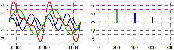 BF=3.5; HF=2.3
g=function(t) sin(1200*pi*t)
h=function(t) 2*sin(800*pi*t)
k=function(t) 3*sin(400*pi*t)
a=-0.005; b=0.005; Piano(a,b, -5,5)
graph2(g, a,b, "black"); graph2(h, a,b, "blue"); graph2(k, a,b, "green3")
f=function(t) g(t)+h(t)+k(t); graph2(f, a,b, "red")
#
Plane(0,800, -5,5)
Segm(600,0, 600,1, "black"); Segm(400,0, 400,2, "blue")
Segm(200,0, 200,3, "green3")
# the freq. are 1/period, ie 1200π/(2π) = 600, …
Other examples of use
BF=3.5; HF=2.3
g=function(t) sin(1200*pi*t)
h=function(t) 2*sin(800*pi*t)
k=function(t) 3*sin(400*pi*t)
a=-0.005; b=0.005; Piano(a,b, -5,5)
graph2(g, a,b, "black"); graph2(h, a,b, "blue"); graph2(k, a,b, "green3")
f=function(t) g(t)+h(t)+k(t); graph2(f, a,b, "red")
#
Plane(0,800, -5,5)
Segm(600,0, 600,1, "black"); Segm(400,0, 400,2, "blue")
Segm(200,0, 200,3, "green3")
# the freq. are 1/period, ie 1200π/(2π) = 600, …
Other examples of use