model and
reality
On some mathematical concepts / themes to be faced in the 1st part of upper secondary school
("interwoven" within teaching units)
[primary - A primary - B lower secondary upper secondary - A upper secondary - B school]
The concept of model
The concept of real number
Non decimal numbering bases
Exponential notation
Powers
Elementary arithmetic
The concepts of ratio and proportionality
The diagrams
Approximations
Calculators. Computer. Logic
Descriptive statistics
Variation and slope
Formulas, terms, graphs
The concepts of function and resolution of an equation
Space
Circular functions
Inverse proportionality
Continuity
Systems of equations. Inequations
Polynomial functions
Exponential function
Mathematical structures
Combinatorics
Theory of probability
Educational differentiations
The same contents present in the document relating to the previous level are more or less faced, with a different slant.
The indications relate to how much should be dealt with in the upper secondary school.
They are presented articulated by thematic areas but, as it is clarified, in the didactic paths the different mathematical concepts must intertwine with each other and with the other disciplines.
In the last paragraph there are indications on the possible diversification of educational development in the various types of schools.
Mathematics can be called the science of models. The concept of model must therefore play a central role in its teaching from the first levels.
The theme of modeling unites all disciplines (examples referring to language education, history, physics, ... are present HERE), also philosophy (think, to make some of the many examples, to the analogies/differences with concept of model of the "ideas" of Plato, Kant, ..., to the interpretations of natural phenomena, from those of the first natural philosophers to those of Galileo, to epistemological and gnoseological reflections). This offers numerous and fruitful opportunities for interactions between the teaching of mathematics and that of other disciplines.
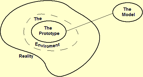
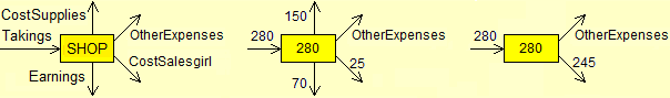
The following figure illustrates the relationship between "model" and "reality". Given a real situation, a model is a simplified representation that illustrates some aspects, for certain purposes. Depending on the purpose there may be different models of the same situation (an airplane model may have the same shape and color as a real airplane but not fly, or it may not resemble a real airplane but fly). The "goodness" of a model depends on its adequacy to the objectives for which it was built (to better highlight some aspects, to generalize some properties, to facilitate comparison with other situations modeled in a similar way, ...). The preliminary phase of the modeling circumscribes the aspects of reality involved in the problem to be studied. Using the terminology developed by Aris (Aris R., Mathematical Modeling Techniques, Pitman, London, 1978) and taken up by Gilchrist (Gilchrist W., Statistical Modeling, John Wiley & Sons, New York, 1984), we can call environment of the prototype the part of reality that is isolated, not in detail, in this way, and we can call prototype the aspects of the phenomenon or situation to be modeled (including assumptions, intuitions, perceptions, intentions, ... of whom builds the model) which will be taken into account in the representation. All of this can be summarized as follows:
| model and reality |
|
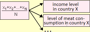
The same model can be used to represent different situations. A very simple example is the concept of arithmetic mean, which can be used to indicate, in a given country, per capita consumption of meat, the average family income, the average height of the twenties, … Another common example is the direct proportionality, which can be used to represent the relationship between the weight of a food product and its cost, between the lengthening of a spring and the weight of the object hanging on it, between the distances among the parts of a car and those among the corresponding parts in a its model, …
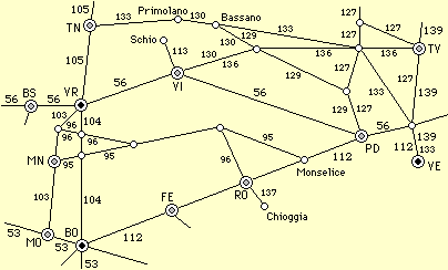
And the same situation,depending on the needs, can be represented with different models. The figure below on the right reproduces part of the graphic index printed on the first pages of a railway timetable: it is a map in which the railway lines are reproduced and the relevant time frames are shown; it is a different model from a usual map in that it does not correctly represent distances and directions.
 |  |
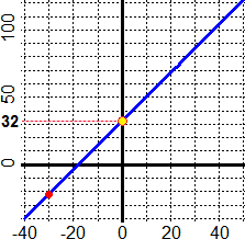
Let's look at another example, simple, in which we face a problem with two different mathematical models. I want to study the link between the DS (S: street) distance along the road and the DA (A: air) distance in a crow line from Genoa to other places in Northern Italy. I can deal with the problem in a conceptual way (understand that when DA = 0 I have DS = 0, that DS ≥ DA, that, given the presence of many curves, the relationship between DS and DA is approximately equal to the ratio between semicircle and diameter, i.e. about 1.5, …). Or I can study the problem empirically (collect data relating to the minimum road distances from Genoa of the provincial capitals of Piedmont, Lombardy and Veneto, and, roughly, correctly using maps or other sources, the data relating to the distances in the crow flie, graphically represent them, try to approximate the points with a straight line, fine-tune how to achieve and interpret this approximation, …). This second approach is illustrated on the side (also with this approach I establish that the relation is, approximately, DS = 1.5·DA; I can then study with statistical techniques which precision to assign to 1.5). | 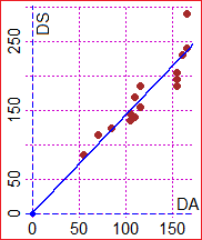 |
Simplifying, we can say that the prototype was the relationship between the distances in a crow line from Genoa to the provincial capitals of Northern Italy and the minimum distances along the road, while the environment of the prototype was generically referred to the distances of Genoa from the various locations. We modeled the problem with the equation DS = 1.5·DA.
In many situations, the model must subsequently be reinterpreted, verifying its adequacy to represent the phenomenon studied and possibly redefining the prototype itself. We can better represent the situation by modifying the previous scheme by adding an arrow
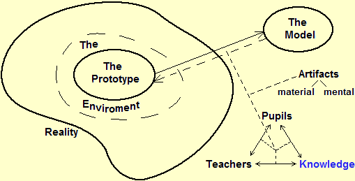
This figure takes into consideration not only the model-reality relationships but also the "tools" used to build the models and how their setting-up interacts with the educational process, that is with the pupils, teachers and the complex of knowledge (the disciplines , the techniques, …).
Models are abstract representations of "real" objects or phenomena (of a material type: a topographic representation is the model of a territory; of a social type: the concepts of "verb", "noun", ... are models for representing certain elements of verbal communication; ... or abstract type: the "commutative property" is a model to describe an aspect of some mathematical operations).
Models are built using cognitive artifacts, i.e. "material objects" (paper, signs, sounds, colors, ...) or ad hoc "artificial constructions" (language, concepts, ...) that man uses as a prosthesis of his mind. The term "cognitive artifact" was introduced by Donald Norman in 1993 (Norman D.A., Things that Make us Smart, Wesley Publishing Company, Addison, 1993), while that of "prosthesis tools" was proposed by Jerome Bruner in 1986 (Bruner J.S., Actual Minds, Possible Worlds, Cambridge, Mass., Harvard University Press, 1986).
The development of cognitive artifacts to model situations does not happen episodicly, but in a social context of cultural growth that is gradually being organized into structured forms of knowledge, which are transmitted from one generation to another through educational processes, in which pupils and teachers interact with each other and with knowledge, the one under construction and the consolidated one. These reciprocal interactions are described by the didactic triangle depicted above which (beyond its repropositions made at the same time, in the early 1980s, by various researchers in teaching: Herbart, Chevallard, …) dates back to Cicero (De Oratore, 55 BC). It was later used also by Quintiliano (Institutio Oratoria, 96 AD), and subsequently by many others. Cicero's idea, in turn, was a reworking of an analogous "triangle", at the top of which were the symbol (or sign), the reference (or meaning of the sign) and the referent (or object to which refers to the sign), developed by Aristotle (Rhetoric, 4th century BC) to illustrate "rhetoric".
What has been observed so far applies to all disciplines and organized forms of knowledge. But mathematics has the specificity of not being characterized by a particular area of problems or phenomena that seeks to model (such as physics, history, linguistics, ...), but by the type of artifacts it employs for the construction of models, and which are used in all other disciplines. So the graphic diagram seen above (which in itself is a simplification) in order to represent the situation of the teaching of mathematics must at least be enriched with the vertical hatch depicted on the side: the artifacts, for mathematics, soon, from cognitive tools become objects of knowledge, from models that "abstract" from situations become gradually "concrete" tools to develop new abstractions, in a never-ending spiral. Mathematical knowledge, which arises from modeled contexts, is organized internally not on the basis of these, but on the relationships and structural analogies between its artifacts. | 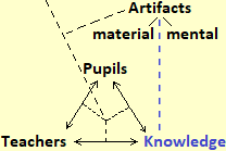 |
The situation, then, becomes more complex as both the "triangle", and the type of "artifacts", with the advent of computer science, have become more articulate: the software has become an "animated" interlocutor that interacts between the different subjects, in ways depending on the use that is made of it and the awareness with which it is used. Without further complicating the previous schematization, it should be borne in mind that the software now has, and will increasingly have, a decisive impact in the way different aspects interact with each other.
[Particular expressions are often used to identify specific cognitive artifacts. These are expressions used in different ways by the various authors, even within the same discipline. We recall some of them, with some possible interpretations. A sign is a cognitive artifact consisting of an "object" which (for a particular community of people) represents a particular meaning or can be a clearly identifiable part of that object (it can be a sign for example the colon, ":", but each of the two points that make it up can also be). A symbol is an object, an individual or another more or less concrete thing used to evoke a real object or an abstract entity; in "mathematics" it is an object constructed with particular signs which represents, in a particular area of mathematics, a constant, a variable, a function, a relationship, …. A signal is an image, a phrase, a sound or an action that serves to communicate a message, an order, …]
|
In summary, however, we can say that the study of mathematics is articulated in the (non-linear) relationship between posing problems, modeling situations to deal with the solution of problems, building and resorting to theories that internally organize the relationships between the artifacts used for the construction of models and develop new artifacts. | 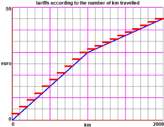 | |
It is necessary to underline one last aspect that the teacher must keep in mind when setting up teaching activities: the difference and interaction between normative models and descriptive models.
Let's consider the fares of a hypothetical bus company. On the right, in red, the tariffs according to the length of the journey:
the graph is a descriptive mathematical object. In blue, a piecewise linear function is plotted:
it is a normative model, which represents the mathematics underlying the tariff, or the "logic" behind it. |
All this makes the role of the teacher crucial in mathematics education. He must:
• design and curate educational pathways that give concreteness to artifacts as they go further away from elementary forms of perception,
• to bring out "reality"-"abstract concept" conflicts (from those between "physical" and "mathematical" mirrors to the many other conflicts present since the first teaching experiences)
They are conflicts that, if not explicit, risk being sources of misconceptions, while, if faced, they are an opportunity to transform a "destructive opposition" into a "productive dialectic", which contributes to building an adequate image of mathematics as discipline.
• educate to the choice of models (there is no "best" model) depending on the needs and "resources" (physical and conceptual artifacts) available,
• organize teaching so that references to real objects or situations are not only pretexts but also establish virtuous relationships with the extra-curricular knowledge (and motivations) of the pupils, decentralizing, trying to have as a reference not only their own knowledge and motivations but, in a dialectical relationship, also those of the pupils,
• and give organicity to the knowledge they have acquired in the mathematical field (even integrating the study of problematic situations with the development - starting from them - of new concepts and the consolidation of some operational skills through appropriate exercises, which depend on the level of knowledge and technologies historically available) so that they become a solid starting ground for new abstractions,
• all this taking into account that, especially in the first levels of education, the building of virtuous relationships with the extra-school also depends on the involvement of "families": it is necessary to make them participate "culturally" in the educational project that is being carried out (participating "culturally" does not mean "to make the repeaters", but to collaborate with teachers in the construction of relationships between school activities and extracurricular life); this is one of the most difficult tasks; this aspect should also be properly included in the "educational triangle" considered above ...
It is only after the start of the construction of the meaning of mathematics as the science of models that the teacher can gradually construct the meaning of the definitions and demonstrations in the mathematical field, focusing on the differences from the other meanings that in the common language have both definitions (in a dictionary they are based on a bank of words - the defining vocabulary - the meaning of which is not explained) and proofs (the proof of the guilt of a defendant is beyond any "reasonable" doubt, it is not "certain"). We shall come back in many other points both to the definitions: HERE, HERE, HERE, HERE, HERE, HERE, and to the proves: HERE, HERE, HERE, HERE, HERE, HERE.
HERE you will find some examples that illustrate the "the limits of the models", including the fact that the identification of a mathematical relationship (statistical, functional, ...) between two real quantities does not always indicate the presence of a cause-effect relationship between of them. These aspects, mentioned earlier (when we observed that the same situation can be represented with different models) and also taken up in subsequent points, are very important to emphasize in teaching.
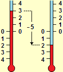
Mastering the decimal representation of numbers should be one of the objectives of teaching in lower secondary school. It is essential, at the beginning of high school, to set up didactic activities that allow to verify this mastery and possibly to start activities that allow you to consolidate it.
In particular, the interpretation of numbers as positions on the graduated straight line must become natural and immediate by pupils: it is one of the few automatisms (of elaboration, association, passage from one representation to another, ...) that everyone must knowing how to perform without mnemonic or reflective efforts (to free mental resources to devote to more conceptual aspects): they are skills/attitudes that should be consolidated/maintained continuously
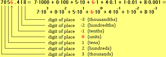
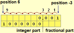
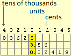
It is also fundamental to consolidate the meaning of the place of a digit and to shed light on how the "reference position" for reading a number is not the decimal point, but the "digit of place 0": probably this confusion is at the origin of the difficulties in reading/interpreting numbers with fractional numbers that some pupils show.
Finally, we observe that we often have to deal with numbers that represent measures; attention must be paid to the misconceptions that can be created by representing these values by means of variables. An example: if I use s to indicate the position in kilometers along the road where I am after t minutes, if after t0 minutes I am 37 km from the beginning of the road and if v is the constant speed in kilometers per hour at which I am traveling, I can write s = v·(t−t0)/60+37; but I have to be careful to always use the same units of measurement. If I used variables to represent quantities, not their measurements in appropriate units, I would have to write: s = v·(t−t0)+37 km.
In the first lessons at the beginning of high school, it is advisable to organize teaching activities that allow you to • explore and review, together with others, basic skills that should be mastered at the end of lower secondary school and, at the same time, • introduce new methods, topics and reflections that also involve and motivate pupils that those skills already master (without isolating, therefore, the "recovery" from new learning).
It is also appropriate to make pupils reflect on the ambiguities with which, in verbal language, numbers with "dot" are expressed (for the importance of this attention to the comparison with common language see HERE), in addition to pointing out (eg by observing the menu options of a computer or mobile phone) the various conventions ("," and ".") which, in the commercial and daily life, are used in various countries to separate the whole part from the fractional part.
For other considerations on the revision and consolidation of the concept of "number", refer to the subsequent reflections on the order of magnitude, the approximate mental calculation, the line of numbers (and the negative numbers), ...; see the following paragraphs up to the "descriptive statistics" excluded.
The mastery of limited decimal numbers, the ability to use graduated measuring instruments, … are fundamental, in particular, to start setting-up the concept of real number, which initially can be called simply number (or unlimited number), postponing the addition of the "real" attribute to when it will be used to distinguish it from complex numbers. It is certainly not a difficult concept: the Babylonians (about 2 millennia BC) already mastered a positional writing system, albeit with a sixty basis (see HERE): e.g. 1 24 51 10 (written using different symbols for the digits) represented the number 1+24/60+51/60²+10/60³; they knew how to calculate the square root of a number with any precision (they had the idea that they could go on and that, stopping at a certain point, they would get an approximation, of which they knew how to evaluate the error); … Textbooks have often gone back several millennia, and with gross errors (see below).
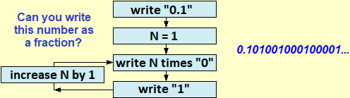
For a correct and meaningful introduction of numbers it is appropriate to choose a constructivist approach; In short:
– real numbers as appropriate sequences of characters (digits, "." and "−"), with an appropriate "equality" relationship (3.7999…=3.8000…, etc.),
– algorithmic definition of operations on limited decimal numbers,
– extension of these to real numbers through the concepts of approximation and (without formalization) of limit/continuous function (e.g. to obtain the result of x·y with a certain precision, it is sufficient to operate on sufficiently small uncertainty intervals for x and for y).
Natural numbers, integers, periodic numbers, limited decimal numbers and those limited in other bases are studied as particular subsets of R which are closed under some operations.
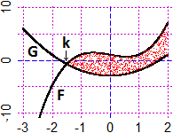
Pupils have already encountered unlimited decimal numbers, such as √2, π, 0.333…, 3.7999… (= 3.8000…, in the early school levels. They have already observed that some numbers, like the last two previous ones or like the one represented in the figure above (0.101001…), can be described exactly, digit after digit, with a simple algorithm, and have discovered that some, like only the first two previous ones, can be expressed as a result of the division between two integers.
At this point it can be focused that this happens for all the periodic numbers (to which it is necessary to focus that also the integers and limited decimals belong), and the words rational and "irrational can be introduced to distinguish the numbers that can be expressed as a fraction between two integers from the others (which are the vast majority).
And it should be stressed that the use of these adjectives ("rational" and "irrational") in this context has nothing to do with their use in the common language (in the meanings of "reasonable" and "devoid of any logic") but it derives from the use of the Latin word "ratio" to indicate the relationship between numbers: in an irrational number it is not said that the numbers follow one another chaotically.
Obviously, it is not appropriate to introduce the real numbers axiomatically, nor to present the construction of the various numerical sets starting from N:
– it would be expensive and difficult to introduce the algebraic-logical-set-theoretic tools to "correctly" carry out the construction (even just the passage) to the integers;
– and, above all, at this level, there are no "didactic" motivations (in a university course of algebra the construction of Q starting from N can instead be an occasion for the application of concepts such as partition, immersion, …) or "cultural" (in a university course on the foundations of mathematics it can instead be significant to construct a model for the axioms of real numbers by set techniques beginning from Peano's arithmetic).
The introduction of the numbers, besides, must intertwine with statistical topics, with reflections on the use of the means of calculation, on the codes, …
In many of the most diffuse textbooks there are serious didactic and conceptual errors. Just think of the introduction of the so-called "absolute numbers" (coupled with absolute radicals and with other nonsenses), the introduction of "+" in front of the positive numbers (among which natural numbers other than 0 are not included!), …, that are only the result of a gross misunderstanding of the nature of mathematics and of a smattering of problems relating to the foundations of mathematics (see the following exercise).
The way to introduce the real numbers presented in this paragraph, from the "foundational" point of view, has clear links with the "arithmetization" of real numbers proposed by Cantor (real numbers and operations between them as "completion by continuity" of the structure of rational numbers), but indeed it does nothing but present the way in which, since the positional notation has spread, we write and work on real numbers (Cantor did not purpose to introduce and define the structure of real numbers, which was already known, but to characterize it, for foundational purposes, as an extension of that of the rationals, and to do it with a procedure that, compared to that of Dedekind, was closer to mathematical practice).
For further information on the foundational aspects (and the cultural motivations of the approach presented here), examine this document: Real Numbers
In textbooks for upper secodary school there is often a caricature of Dedekind's approach: real numbers are introduced as elements of separation between contiguous classes of rational numbers, without realizing that, if I do not already have real numbers, it does not exist any element of separation except in cases where it belongs to one of the two classes, and is therefore rational; and the problem is not posed that, however, one should find a way to connect (and in a "correct" way) this "construction" to the usual way of writing numbers For the errors and inaccuracies that generally stud these "treatments", compare them with the trace of a correct "Dedekind" development (and which can only be tackled at university level) that can be found in the document accessed from the previous link.
The first non-decimal bases to be introduced and that the pupils must master are those used in the measure of time (bases 12, 24, 60), on which they have operational skills acquired gradually over the course of their life. The task of the teaching is to manage the transition from these skills to the explication and formalization of the ways in which to move from one of these bases to base ten, and vice versa, and on how to operate between numbers expressed in these bases, not by introducing abbreviated mechanical rules, but procedures and forms of description that do not cut the links with the ways of operating in daily life and that do not obscure the references to the concepts of "ratio" and "change" of units of measurement.
Consolidated the analogies between base ten and base sixty and the ways in which to pass from one to the other, the context of the coding of numbers in electronic devices (and that of reflection on the "strange" outputs of the computing means) could constitute, later on, the occasion and the motivation for an extension to other numbering bases.
A precocious approach to a general treatment of the bases of representation of numbers, especially if initially referred to bases which are not used in everyday experiences,
− is didactically counterproductive:
• explication and reflection on operational skills acquired experientially are fundamental,
• their consolidation through the development of methods that help to cope with difficult situations for mental calculation,
• the individuation of analogies between different situations and the usefulness of their conceptual unification,
• the acquisition of the habit/ability to relate to examples and prototype situations to reconstruct general concepts and methods (habit/ability difficult to acquire without going through the previous sentences),
• ...
− and it offers neither cultural motivations nor an adequate image of the nature of mathematics.
| It is important to immediately introduce the use of exponential notation and focus on its usefulness, together with the consolidation of the use of different units of measurement and of the positional writing and with the education in the use of pocket calculators and to the mental development of the approximate calculations. | |
| In addition to the convenience of exponential notation for describing large and small numbers, it is good to highlight the fact that it facilitates syntactic and semantic control over what is written, that using it to introduce numbers with orders of magnitude large or small on a calculator makes it more difficult to make typos (e.g. forget some zeros), that it allows an unambiguous description of the approximations. The latter observation can be developed explicitly when, in subsequent school levels, a more systematic study of "numbers" will be tackled. | 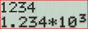 |
| The "statistical" themes offer many opportunities to naturally insert the first activities and reflections on the use of exponential notation and (see below) the use of powers. | |
Mastery of exponentiation is fundamental in the most varied fields of mathematics.
It must be verified, consolidated and deepened starting from the first years of high school, not through activities detached from contexts, but in relation to situations of use in which the powers intervene significantly and which can constitute solid points of reference for the conceptualization and memorization. The reference to the powers of 10 is fundamental in this regard.
On the other hand, activities with powers (if they are not immediately reduced to the mechanical application of rules) can help consolidate the meaning of negative numbers and additions with them. E.g. this is possible if in the explanation or correction of errors in calculations such as that of
|
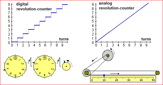
In resuming this concept, already started in previous schools, it is appropriate to make some initial reflections on the "definitions": in the definition of the power with integer exponent, the exponent indicates the quantity of times, starting from 1, multiplications (or divisions, if the exponent is negative) for the base are carried out. This definition, which "translates" and extends the usual recursive definition (a0=1, an+1=an·a), is immediately connected to the concept of order of magnitude (exponent of the power of 10 of scientific notation). It also corresponds to how the calculation is performed with a "for" loop: a=3; n=7 p=1; for(i in 1:n) p=p*a; p # 2187 a^n # 2187 |
 |
Recall that in many books the following definition is widespread: "an is the result of n multiplications of a by itself", which is obviously wrong (if we start from a instead of 1 the multiplications for a are
It is appropriate to point out to the pupils, when indicating a succession of operations of the type
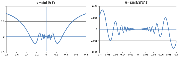
On the extension of powers from the case of the whole exponent to those of the fractional exponent (within which the study of radicals must be addressed: they must not be studied as objects independent of powers, with their rules and properties) and, then, those of the real exponent (in particular, to give meaning to the treatment of graphs such as that of
Obviously, in the activities mentioned above, the meaning of the 4 operations must be resumed and consolidated (relationships between them, situations of which they are models, geometric interpretation, .…). These observations and reflections, carried out on several occasions, can be explicitly taken up in a unitary way, to consolidate some basic concepts and skills, and also to create the conditions for subsequent didactically effective interventions towards pupils who will manifest difficulties in setting-up the equations. It is useful, in particular, to discuss their mental calculation strategies with pupils, questioning them if incorrect, proposing alternatives, … but without setting the objective of imposing on them procedures other than those they employ, if correct: different people can, for various reasons, prefer to follow different types of reasoning.
If it is of use, it is good to resume the basic elements of the 4 operations techniques, recovering mental and non-mental calculation skills, often obscured by "fast" (and "volatile") techniques on which the pupils were trained in the previous school levels (see HERE to get an idea of how "calculation techniques" should have been introduced in primary school and, in case, resumed at the beginning of secondary school).
It is also necessary to keep in mind the possible presence of pupils with dyscalculic disorders. Dyscalculia is present in about 2% of the population, therefore in a class of 25 pupils in basic school there is about 50% probability of having a pupil with a pupil with such problems; the probability of having two is much lower, around 25%; of having three is about 10%. A primary school teacher during his career should meet about 5 pupils with dyscalculic disorders (often, due to the incompetence of those who make these diagnoses, situations that do not fall within this area are reported as dyscalculic cases). A lower secondary school teacher might meet about ten.
For high school teachers, the number depends on the type of school in which they teach.
What to do in these situations? First of all, it should be noted that dyscalculia occurs in pupils with normal intelligence and without neurological disorders. It is therefore necessary, starting from the basic school, as with the other pupils, to refer to all the real life situations in which numbers are used, to refer to algorithms in which the meaning of the procedure is transparent and, in particular with them, to rely immediately on technological aids for carrying out the calculation activities, initially limiting their use by other pupils.
You can use the usual calculators or calculators present in the software, such as those that can be accessed from HERE; you can use the Google "translator" (see HERE) where you can write numbers and operations (such as: 7.5 1500 12% 5000000 3/4) and listen to their reading; you can also (as suggested by the international website dealing with dyscalculia) use WolframAlpha (see HERE, then click on Elementary Mathematics, Arithmetic).
Dyscalculic difficulties are largely related to memorization problems (similar in some respects to similar difficulties that can occur in some people following accidents or small strokes) that do not compromise the understanding of mathematical activities if you rely on the use of the computer,, as can be done for several decades now. Obviously, teachers should stimulate these pupils, from the early years of school, to use the means of calculation suitably.
A similar in many ways (and slightly more frequent, about twice the dyscalculia) disorder is dyslexia, i.e. the difficulty in reading and sometimes writing words, which usually occurs with the transposition and inversion of groups of letters. The use of the computer is obviously also of great help in facing the problems it generates. You can resort (similarly to what was said for dyscalculia) to Google, to free writing programs (such as OpenOffice, LibreOffice, ...) and to their spellcheckers (which offer alternatives to what has been typed). The same typing of texts on the computer, and the observation of what is being written, and the possibility of correcting what is written, is in itself helpful for those who have problems of this kind.
The activities on the line of numbers, in particular those involving negative numbers, are very useful for consolidating (also through the repetition of similar exercises) the habit of leaning on the (mental image of the) line of numbers. It is important to introduce negative numbers correctly, not to use rules (harbingers of misconceptions) such as "−" by "−" make "+", not to put the "+" sign in front of positive numbers, ...; frequent errors resulting from these misconceptions are, for example, that of transforming
On the first traces of the use of negative numbers by the Babylonians (which we have mentioned while discussing the "arithmetic operations") considerations can be found in various books by Martin Gardner and in many scientific articles; for example see HERE.
It is useful: • to interpret the errors or difficulties of (written or mental) numerical calculation of the pupils, • to make its origins explicit, • to get them do checks on the properties erroneously used (or those not used) in simple cases, • to resort to geometric interpretative models for generalize numerical examples, such as the following (the first illustrates a usable property, the second an error):
 |
Operations with negative numbers are easily understandable, if introduced by interpreting the "negation" as a reversal of direction. For example, in the case of the formula |
 |
These reflections/activities should make it easier for pupils who encounter difficulties in the face of more formalized reasoning to understand and internalize the transformations to which a numerical term can be subjected. It is useful, subsequently, to introduce, in an operational way, graphic representations of the structure of the terms.
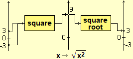
|
|
       +
   ___/ \___
SQR         /
 |      ___/ \___
 2     *         C
    __/ \__
A B |
       +
   ___/ \___
SQR         /
 |      ___/ \___
 2     *         C
    __/ \__
A B |
       +
   ___/ \___
SQR         /
 |      ___/ \___
 2     *         C
    __/ \__
A B | ||
| square root | multiplication | division |
Note. Arithmetic operations are the first numerical functions with which one has to do in school life. After a first start, in which one becomes more confident about using operations and starts the formalization of the functions, it is necessary to frame the operations in this more general concept. The term operation in mathematics is used in different ways in the various areas of the discipline. Generally it indicates a function (or application) described through a procedure (in a broad sense, not necessarily "mechanical") and which takes on particular importance in the characterization of a certain type of mathematical structure or of a particular sector of mathematics; the functional symbol used to describe it is called operator, but sometimes this term indicates the function itself. Examples: the union between two sets (it is an operation that associates another set with two sets, and which gives a certain algebraic structure to the class of subsets of a certain set), the composition of functions, the passage to the limit, derivation and integration, scalar and vector products, … See HERE for some further notes.
In the development of mathematics teaching in its various areas, it is important to gradually highlight (occasionally, without dwelling too much) analogies and differences between ways of working on numbers and ways of working on other mathematical objects. These scattered considerations can gradually build the ground on which, then, between the end of the two years and the beginning of the three years, set (in the not too "difficult" classes) a more organic setting. We will return to these aspects later: see formulas, terms, graphs and mathematical structures.
The concepts of ratio and proportionality
Much of the first year of upper school should be devoted to laying solid foundations regarding the mastery of numbers (in base ten), the concept of ratio, the concept of function, the use of graphs, the use of variables, terms and equations to represent relations between quantities, to the representation of algorithms. Shifting attention to secondary aspects or new concepts that at the moment can only be addressed with erroneous presentations (as happens for example in the usual introductions of polynomials, not related to the concepts of function and equation) or with mechanical and superficial learning (the literal calculus without an adequate understanding of the meaning of literal language and of symbolic calculus and of the role of algebraic modeling; the calculus in non-decimal bases without mastering the concepts of relationship, coding; ...) would be counterproductive.
In particular (within the didactic paths where the other concepts mentioned above are present) it is appropriate to resume, consolidate and extend the mastery and knowledge of the concepts of ratio and proportionality (direct - on the inverse one see below inverse proportionality).
It is essential that it is clear to the pupils that "%" signify "/100", that they know how to express percentage variations as multiplications (10% increase as multiplication by 1+10/100 = 1.1, 20% decrease as multiplication by 0.8) and that set calculations in this way with calculators: this is important for focusing that subsequent percentage changes are not made by adding them up, that, once an increase of P% has been made, a decrease of P% must not be made to return to the initial value, that the variation of P percentage points is not equivalent to a variation of P%.
The considerations carried out evidently refer to the use of the concept of function, which must be used constantly, taking up again (in an operational way) the knowledge developed in the basic school.
The graphic representation of (direct) proportionality and of phenomena in which the variation of one quantity is proportional to that of another provides the natural context in which to move from the "physical" to the "mathematical" slope (see variation and slope) and resume and make clear the concept of linear function and the link between graphic and symbolic solution with respect to x of the equations of the type
It is also a very natural context for the recovery and consolidation of the first formula manipulation activities.
We emphasize the awkwardness to resort to specific resolution techniques for proportions (instead of considering them equations like the others) to deal with proportionality problems.
If some pupil, by heritage from previous "bad" teachings, proposes proportions of the typeo
   angle    datum               datum
  —————— = ——————  —>  angle = ——————·360
    360     total               total
To draw various types of diagrams (variation and slope) it is necessary to focus on the role of scale factors. This is a very important aspect, not only for the interpretation of the graphic representations of statistical data (and to introduce considerations/attentions that will be useful for the construction and reading of the graphic representations of statistical distributions referring to intervals of different amplitude), but also to master the units of measurement of areas and volumes and the transition from one unit to another, and to make estimates. It also comes into play in many other issues of Physics and Biology, as well as of Mathematics. | 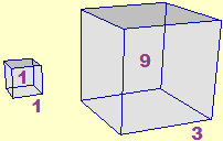 |
The concept of fraction should be presented as a particular case of ratio: this allows the different aspects in which fractions meet in applications to be well intertwined. The "algebra of fractions" can be discussed later (see mathematical structures): first it is necessary to focus on how to compare ratios, how to determine the reciprocal of a ratio and, then, on the use of distributive property (see formulas, terms, graphs).
Obviously, the context of proportional representations also offers simple and significant opportunities to educate the use of software tools for the partial or total automation of calculation procedures.
As it should happen for the introduction of all mathematical models, it is good that even in the case of the concepts discussed here,
not only the advantages of their use, but also the limits, are highlighted:
the information that is lost by comparing percentages instead of absolute data,
the care with which the comparisons between the evolution of different phenomena based on their representation by means of index numbers or relative variations must be interpreted, ...
If, for example, a spreadsheet is used, it is necessary to warn against the errors of representation/interpretation that can induce a non-critical use of its menus (see here).
The use of the various graphical representations (line of numbers, graphs, tree graphs, histograms, schemes, ...) greatly facilitates the reasoning, the framing of the problems,
the research and conjecture of solution strategies, the exploration of connections , relationships or regularities, the display of large quantities of information,
the development of models that allow easy passage between context and concepts with which it is mathematized, ...
It is also the way in which mathematical elaborations (relating to sociological investigations, economic situations, technical-scientific phenomena, ...) are generally communicated to us by the mass media.
Graphical representations are increasingly present in the various sectors of mathematics.
And many of the more abstract concepts are born as generalizations of spatial concepts, of which they carry the traces, metaphorically, in their name
(spaces of functions, spaces of infinite dimensions, metrics on abstract spaces, measures of abstract sets, ...
and points, coordinates , diameters, projections, orthogonality, ... referring to objects that we cannot physically represent).
It is therefore fuamental that the teaching educates the use of graphic representations (both to model situations and to carry out theoretical considerations), to the transference between them and other forms of representation, to the intertwining of graphic methods and symbolic and numerical methods, ...
It is appropriate that from the first lessons (intertwining with considerations of statistics, geometry and analysis of various phenomena) the main forms of graphic representation are introduced, highlighting their potential, limits and interpretative problems (see, on the right, different representations of the thousands of unemployed over the years). Specific insights on the Cartesian plane and on the curves can be carried out later. | 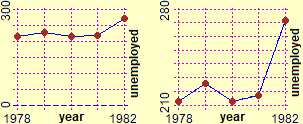 |
The computer is an extraordinary tool that facilitates the construction (and reading) of many types of graphic representations.
There is a lot of free software that can help in this regard.
However, it is important that pupils first learn to draw graphs by hand, starting from both data and algebraic representations,
that they acquire the ability to sketch, with the necessary accuracy depending on the context, the graphs of the main functions as they are studied, ...,
and that they become able to imagine graphs, to describe them in words, ..., as well as to graphically schematize problems, graph terms and procedures, to associate graphs with phenomena, ...
The topic "approximations" must be introduced gradually within all the didactic activities, without an autonomous treatment, since according to the contexts there are various ways in which it presents itself: reading and interpreting approximate data that they are found on articles, on television, …; distinguishing the different more or less formalized ways in which approximations are presented; knowing how to read measurements with the various instruments and describe them mathematically; understanding the difference between rounding and truncation approximations and the different ways to work with them; approximating the results of operations and of various procedures obtained with a calculation medium (on this aspect see also Calculators. Computer. Logic); reading and graphically representing information that depends on approximate data; …
The theme must then be taken up again in the last years of upper secondary school, connected to more general mathematical themes (the differential calculation, the approximations of curves, the approximations of probabilistic calculations carried out through statistical simulations, ...), as well as to physical themes (to have a idea of the connections with physics see HERE).
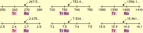
We recall here the current meanings of truncation, rounding and significant figures:
| |||||||||
The last example above also highlights the usefulness of exponential notation: to clarify that 1400 is the 3-digit rounding of 13.961 (not just the 2-digit one) we can express ourselves using the scientific notation 1.40·10³. However, it is also necessary to point out that a means of calculation does not put the final zeroes …
Some technical clarification.
The mathematical term rounding, to be rigorous, was not born as a synonym of "approximation to the nearest number (integer or ...)",
but to indicate an approximation with a lower number of digits (as also the etymology of the word suggests ).
However, in recent decades this interpretation has spread, to clearly distinguish "rounding" and "truncation".
Note, however, that the word "rounding" is often used even in the broadest sense; for example, speaking of errors or rounding problems in the automatic calculation,
one refers to the phenomena resulting from the approximations with fewer digits made by the machines, regardless of the way in which these approximations are carried out.
The concept of significant figures is often used even in a broader sense.
For example, it is said that 4.52 is a 3-digit rounding even in situations where it refers to a number between 4.51 and 4.53 (not between 4.515 and 4.525 as was done here):
if a balance is guaranteed with a precision of 1 gram and gives 160 g as weight, it can be said that it has 3 significant digits, meaning that the weight is
160±1 g, ie it falls in [159 g,161 g]; if the balance had a precision of 10 grams we would say that the weight 160 g has 2 significant digits,
meaning that it is 160±10.
We could also approximate to the nearest fifty: 1867 would be rounded to 1850 and the significant numbers would be 3 (185)..
More generally, sometimes one speaks of n significant digits even in the case of an approximation in which
we have some information on the initial nth digit, that is, in which one only knows how to delimit the values that the nth can assume initial digit
(for example if the value 34.6178 is obtained and we know that the error does not exceed 0.03, we can infer that the 4th initial digit cannot be any digit:
the number must end with 58, 59, ..., or 64; we cannot say anything about the 5th initial digit; sometimes, therefore,
it is said that the significant digits are 4, i.e. 34.62, although to be precise we could only write 34.62±0.04, so as to understand the whole range 34.6178±0.03).
It is important that pupils are stressed that it is convenient to make roundings only at the end. It is, however, a habit to be consolidated through practice (and the reasoned use of the means of calculation, right from primary school). At one time (until about 1970) when proceeding with manual calculation, it was more convenient to operate on rounding of the intermediate results, even if the precision of the result worsened. Such things, however, half a century later, are still found in many manuals of both physics and mathematics!
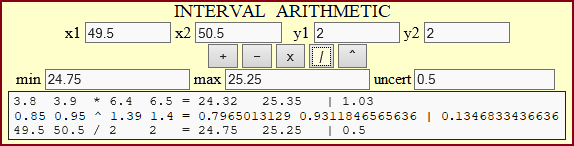
Given the approximations for excess and defect of the data, you can automatically find the approximate result of the 4 operations and of the exponentiation by finding the minimum and maximum of the 4 results obtained by operating on the different approximations with a simple program; here for example what can be achieved with this, executable online (a rectangle with sides between 3.8 and 3.9 cm and between 6.4 and 6.5 cm has an area between 24.32 and 25.35 cm², with an uncertainty of 1.03 cm²; if I know that x = 0.9±0.05 and that y is between 1.39 and 1.40 I can conclude that xy is between 0.7965 and 0.9312, with uncertainty 0.1347; half of 50±0.5 g is between 24.75 and 25.25 g, with uncertainty of 0.5 g; the uncertainty is the difference between the two approximations).
In more complex cases, the random number generator can be used to find the result with a numerical experimentation, in a more precise and reliable way than with the differential calculation techniques often used. See for example HERE.
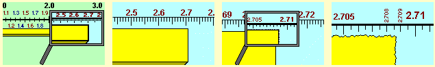
|
Graduated instruments are generally constructed in such a way that the amplitude of a division corresponds to the sensitivity of the instrument,
that is, to the minimum variation of the measured quantity which causes the value indicated by the instrument to vary; in these cases precision
and sensitivity can be considered as synonyms.
But this is not always the case: in some cases it is enough for the instrument to perceive a small stimulus for the indicated value to change by more than one division;
a similar phenomenon often occurs with the instruments in which the measurements are expressed digitally:
for measurements of a certain order of magnitude at the smallest variation the last digits vary by many units
(in these cases the accuracy of the instrument can be much greater, i.e. much worse, compared to the value that corresponds to the variations of the rightmost digit),
while for measurements of other orders of magnitude the same instrument can behave in the opposite way (the last digit clicks more slowly than the variations that the instrument actually perceives). | |
|
In physics, a distinction is often made between precise measurement and accurate measurement: a measurement x of a quantity x with uncertainty
|  |
It is opportune, from basic school, to make extensive use of pocket calculators. It may be useful for the teacher to review the models available to the pupils (for example he can ask the pupils to draw the keyboard of their calculator on a sheet). It is also appropriate to invite the pupils to read the user manual of their calculator (initially excluding the keys for more complex functions). We remind that the use of calculators is indispensable if there are pupils with dyscalculic difficulties, as mentioned in the item elementary arithmetic.
The objectives should be eiher to acquire a greater mastery of this means of calculation, to understand its limits in order to interpret the results it provides, …, or to introduce and/or consolidate (at a first level) some mathematical knowledge: numbers (approximations, real mumbres, …), on functions (functions with multiple inputs and multiple outputs, composition of functions, inverse functions, …, set of definition, …, circular functions, …), …, or to prepare the ground for understanding the functioning of computers (which, as mathematical knowledges and arithmetic calculation possibilities. do not differ "essentially" from a pocket calculator).
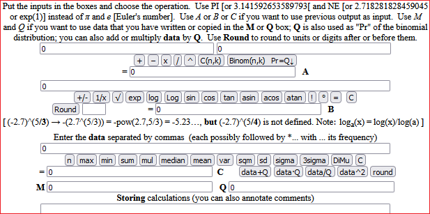
It is evident that the use of the means of calculation is to be introduced and developed at the same time as the treatment of the other mathematical themes, albeit with specific insights. Examples of activities in this direction can be suggested by the exercises present HERE (and in the following pages), in which the theme is enlarged to that of the description of the algorithms and to the description and reflection of various aspects of the automation processes, a theme to which − given the centrality it has assumed in the normal work of almost all mathematicians and those who use mathematics in other disciplines, techniques or professions − an autonomous space must also be given, which can subsequently suggest further mathematical developments; some ideas in this sense can be suggested by the material present HERE. Some examples of various types of software can be found HERE. An example below: a "pocket calculator".
Starting to use programming languages and other software also involves discussing the analogies and differences between formal and artificial languages.
A related aspect is the discussion of which aspects of the Logic theme can be addressed at school level;
this theme can only be interpreted in a broad sense, as education for attention to linguistic aspects, to understandable presentation of arguments, ….
Logical operators are to be understood as elements necessary to construct functions and relationships to be formally described and elaborated,
certainly not as elements to construct formulas to be studied in the context of formal logic, an area of mathematics that cannot be addressed
(if not caricaturally) in pre-university studies (see HERE).
It is worth mentioning that even demonstrations cannot be included in a specific area of learning: they are widespread in all areas of mathematics,
and the demonstration techniques (and the ways in which the mathematical propositions to be demonstrated are expressed) are very numerous,
not enclosed in some stereotyped examples, as often happens in textbooks (a reflection on what the demonstrations are can be found HERE;
some examples of activities on the area of logic and demonstrations can be found HERE, and in the following pages).
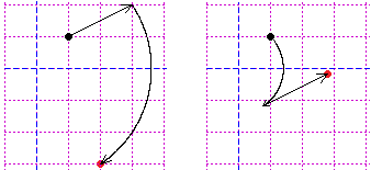
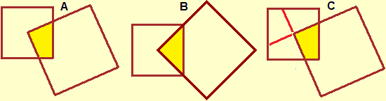
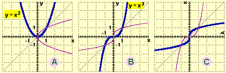
As already observed for lower secondary school, the differences between intuitive arguments and demonstrations must be focused. For example in the following case where the big square has a vertex in the center of the small square (figure A) I can assume that the part that the two squares have in common is about a quarter of the small square, I can believe that things are exactly in this way thinking about fact that by rotating the big square I can get to figure B, but to demonstrate that this is valid in general I have to do the reasoning illustrated in figure C.
And, as already noted, we need to worry about the construction of concepts and mathematical language, and the meaning of definitions, rather than about the memorization of some definitions, often wrong. Clamorous are the wrong definitions of parallelism spread in many textbooks: see here.
Furthermore, the conflicts between mathematical terminology and common language, especially in the geometric field, must be highlighted (also at the beginning of the upper secondary school): the different meanings of angle, direction, distance, curve, ... and of many frequently used words; for example, in normal communication when we speak of a rectangular table we mean one that is not square, while in mathematics rectangles are particular squares. This also sends back to the way in which the concepts are defined: if I say that an isosceles triangle is a triangle that has two equal sides meaning that the equilateral triangles are also isoscosceles, I take for granted that "two" stands for "at least two", not for " exactly two "; for the "educated" adult this is obvious, for the student not; the teacher must explore the possible existence of misconceptions of this kind. Think also of the many meanings that the equal word has in mathematics, completely different from the profoundly incorrect ones attributed to it by many books ("equal" as "being the same thing"): see the many examples presented here.
Note. If the teacher wants, he can put graphics on the net made with a simple script and that pupils can freely resize with the mouse (see HERE):
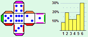
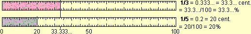
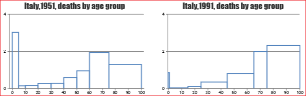
Descriptive statistics (to which we have mentioned several times discussing the previous topics, and in particular the concepts of ratio and proportionality) lend itself to the introduction in significant contexts of many basic mathematical concepts, from numbers to approximations, from the concept of function to the construction and use of formulas, from graphic representations of numerical relationships to the reading and development of algorithm. This, at least, if it is not reduced to being an additional theme to be taught separately from the other themes. The descriptive statistics tools then serve as points of reference for the subsequent introduction to probability (concept of distribution, property of the probability-function, ...). HERE are links to programs that can be used for statistical processing. We mention a couple of important observations to face with the pupils. The first is that the sum of three or more approximate percentage frequencies is not necessarily 100: if I have a total of 150 divided into three parts each equal to 50, the percentage frequency of each of them is 33% or 33.3% or ...; their sum is not 100. The second is that there are several concepts of "mean" in addition to the arithmetic mean. In addition to the very important role of the median it is important to focus on that the average speed is not obtained by doing the arithmetic mean of several speeds. | 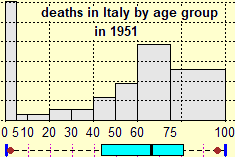 |
It is also appropriate to focus that in a histogram (like the one above on the right) the frequencies of the various classes are represented by the areas of the rectangles, not by their heights! This aspect will be important, successively, to face in the following classes (without misconceptions) the study of continuous random variables using integration (if the distribution is represented by a curve, the probability that the output is between A and B is the area under the graph between abscissas A and B).
The contexts to which statistical surveys can refer are innumerable. However, it is also appropriate to refer to issues close to the cognitive (and psychological) needs of boys and girls of this age group (society, body development, school, ...).
Other statistical activities can also be carried out within the physical chemical laboratory.
However, it must be borne in mind that they can only make sense in the context of highly sensitive measuring devices:
the usual measuring instruments for lengths (meter, caliber, palmer, ...), for weight (spring balances and the like), for temperature (thermometer),
for time (clock, stopwatch, ...) ... are low sensitivity, i.e. the uncertainty coincides with the sensitivity of the instrument
(i.e. with the maximum appreciable difference using the graduation or the figures displayed).
It makes no sense to make statistics on measurements so carried out which, if the survey is made with care, must repeat themselves identical
(or at worst with an uncertainty on the last digit in the case of measures that are halfway between two notches - if we're rounding off - or around a
notch - if we're truncating).
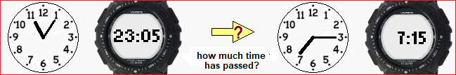
The measuring device for time intervals consisting of a stopwatch that detects hundredths of a second, but which is operated by hand,
can be considered a highly sensitive instrument: in this case, the component of the apparatus that governs the start and stop causes
random errors to come into play which have an order of magnitude greater than the sensitivity of the stopwatch, so it may be appropriate
that the measurement is carried out simultaneously by several people and then a statistical analysis of the various measurements is made.
One can then choose a pair of percentiles to be taken as extremes of the uncertainty range, for example the 25th and 75th percentiles
(this choice corresponds, roughly, to the idea of taking the range of values such that, if make a new measurement,
there is a 50% probability that it will fall into it).
The topic is to be taken up and deepened in the second part of upper secondary school, using probabilisitic concepts.
At the beginning, therefore, it is good to operate, even in the physical-chemical field, with low sensitivity measurements.
We have already discussed the introduction of these concepts several times when we reflected on the development of the concepts of ratio and proportionality.
It is fundamental to weave all these concepts into the graphic representation of proportionality (and linear functions), to highlight the diversity between absolute and relative variations, to focus on how the latter are representable/interpretable as products, ….
10% increase 20% increase x ————————————> x�(1+10/100) ————————————> x�(1+10/100)�(1+20/100) = x�1.1�1.2 = x�1.32 |
This work serves, moreover, to build conditions for the solution of equations, for the study of geometry,
for the introduction of elements of three-dimensional geometry and, finally, for the introduction of the concept of "derivative".
We have talked about variables, constants, terms several times in the previous paragraphs (in particular under the items model concept and elementary arithmetic) and we will talk about them in the following ones (starting from the next), since they are concepts and linguistic aspects of basic (related to the writing, interpretation and modification of the formulas), to which, anyway, it is necessary to give, at a certain point, a first set-up, decidedly different from the "funny" way of starting the algebraic calculation often used in textbooks (introduction of strange things called polynomials, which are not [see the entry polynomial functions], lack of connections with the uses to represent and solve equations, ...).
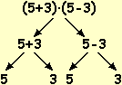
We remember the importance of recalling from previous school levels, or of introducing, the use of "tree graphs", important for learning the meaning of formulas, learning to switch from one language to another, reading formulas not only as sequences of symbols, strengthening the first conventions in the writing of terms, ... and describing procedures that cannot be easily described as formulas, solving problems, ...
We need to focus heavily on the analysis of the structure of terms,
thinking that difficulties related to this aspect are at the origin of many of the most common mistakes of pupils.
Furthermore, pupils must be encouraged to identify, make explicit and control the transformation processes from time to time used in the various passages.
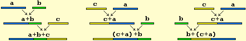
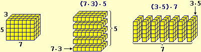
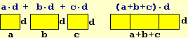
The aim is not to demonstrate all algebraic transformation processes to pupils; for example, rather than associative property, it is better to focus directly on the
"property of reordering" (illustrated in the first two following figures), which would not have been trivial to demonstrate starting from associativity and commutativity
(two properties which, on the other hand, would in turn require a very complex justification, referring to the algorithms for the operations, or an axiomatic justification).
The objective is rather to have the algebraic calculation carried out by having clear the sub-terms on which one operates,
also initially by making the terms represent by tree graphs, and highlighting clear contexts (generally of a geometric type) that justify the basic properties.
It is also important to note that graphic methods allow you to anticipate, and then motivate, algebraic techniques. An example:
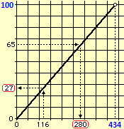 |
Which "percentage" of 434 is 116?
        dat            65    dat
   65 = ———— ·100  →   ——— = ————  →
        434            100    434
    65                       65·434
   ——— ·434 = dat  →  dat = —————— = 282.1
   100                        100
|
For some historical and didactic considerations on the use of formulas and on elementary algebra see HERE, where some coarse errors often present in the definitions found in school books are also commented.
For some reflections on the "=" symbol and its different uses in mathematics must also find space in teaching, to avoid or overcome misconceptions. See HERE for some examples and some didactic considerations.
We observe that some textbooks speak of arithmetic roots. It is a strange concept that has little to do with the concept that, at one time, was used to identify with this term, to distinguish it from algebraic roots: with the first it was indicated that it is simply called "root", with the second it was indicated the set of solutions of an equation (with unknown x) of the type xn = k; e.g. in the case of x2=4 we would have {−2,2}. In these books the root of nonnegative numbers is called arithmetic root. So
The concepts of function and resolution of an equation
The concepts of function and equation are perhaps the most important concepts of mathematics; they intertwine with almost all the other voices discussed here. They are present in programs of all school levels. Evidently these are concepts that are upstream of the concept of polynomial and it is surprising that in many textbooks this is introduced earlier (on the manner, unfortunately funny, in which this introduction takes place we dwell in the specific paragraph polynomial functions).
The first functions that the children explicitly meet are, at the beginning of primary school, the four operations (two inputs), the unit increase, the unit decrease and the change of sign (one input). But in primary school they also encounter functions with any quantity of input, such as the maximum and minimum of a set of data, and functions to which a calculation procedure does not correspond (for example the height or weight of a person, or the population of a city, as a function of time; or tariffs of various kinds, in which the monetary value is expressed as a function of various quantities). They also meet with multi-output functions (division with remainder, for example, is a two-input and two-output function).

On the other hand, even the histograms with crosses (which can be introduced before elementary school, in kindergarten, like those present HERE) are functions: every way of getting to school is associated with the number (represented by a column of crosses ) of the pupils who use it; each type of holiday resort is associated with the number of pupils who spent it that way; each weather condition is associated with the number of days of the month in which the weather was such; …
It is evident that these concepts have little to do with the definitions with which they are introduced in many textbooks: a function is a set of ordered pairs such that …; the authors of these books have picked up definitions like this that are done in university algebra courses, without realizing that in order to master them one must have techniques, not at all simple, to represent an input sequence and an output sequence with a suitable pair of mathematical objects.
It is necessary to adequately construct the possibility and the opportunity to present the functions as sets of
Recall that the name "operation" is an appellation used to indicate some functions, generally with 1 or 2 inputs, but not only. There is no "definition" of the concept of operation.
It is important that pupils consolidate the "concept" of function (not that they memorize a "definition" of it)
by referring to various ways of expressing or representing it (numerical, graphical, algebraic, in words, …),
by gradually strengthening, whenever possible, the intertwining of these ways.
It is essential that pupils immediately resume and consolidate the meaning of square root (which can only be defined, since the beginning, referring to the real numbers,
intended and introduced as decimal numbers, the numbers that are used and whose meaning is to be taken up again from middle school:
rational numbers - not fractions - obviously must be introduced later, as a substructure of real numbers, which enjoys particular algebraic properties).
Students must then be accustomed immediately to represent graphs of continuous and discontinuous functions (without introducing specific terms to distinguish them)
in order to avoid that they tend to identify functions with only continuous ones.
Obviously, the use of pocket calculators and, later, that of computers are decisive in our day; for them we refer to a specific item.
It is good to indicate the variables in various ways, as happens in everyday life. These uses must then be followed gradually by exercise and abstract consolidation, which can be done on variables with names that are independent of the various application contexts. And it is good to realize immediately that a formula can be transformed by expressing a variable as a function of others in different ways, depending on the needs. It is also essential to refer to the concept of inverse function, as a tool for disassembling/transforming equations.
It is important that the teacher, especially in the initial phase, uses informal ways of expressing himself and, when resorting to more formal or formalized expressions,
he does so with a certain rigor: certain incorrect uses learned at the beginning are the source/nutriment of profound misconceptions which, then, is difficult to disassemble.
For example it is good to point out that if F is a function
The reflections on the concepts of function and equation are often intertwined with the use of software, for calculation and for graphic representation; if one does not have a computer room, classroom presentations can be made on how it can be used, leaving the students to use it at home. Those who cannot use the computer room but have calculators or pocket computers with a graphic screen can carry out similar activities using the graphics programs incorporated in these calculation means; otherwise: pocket computer for calculations and ... graph paper and pencil!. However, paper and pen are also indispensable to use the proposed software: both to write down data, expressions, ..., and to take notes while "thinking" about how to use it (individuation of strategies, choice of commands and data to be introduced, ...): programs are only a "subsidy", although sometimes indispensable.
It is necessary to illustrate or exploit didactically the analogy of the schematizations of the composition of functions with the use of graphs and diagrams in different areas, considered in other entries.
 | 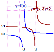 | 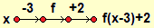 |
It is necessary, immediately after, to focus on the analogies and the differences between the functions x → xn with n even integer and those with n odd integer, in relation to the symmetry with respect to the vertical axis or with respect to the origin of the axes, and in relation overturning around the bisector of the first quadrant.
The procedure of "applying the same function to both members" to solve equations should be gradually introduced, without initially investigating its limits.
(A-2)/5 = 1/4   I apply u → u·5
    A-2 = 5/4   I apply u → u+2
      A = 5/4+2 = 4.25
|  | √(2x+5) = x+1 I apply u → u²
2x+5 = x²+2x+1 I apply u → u-2x-1
4 = x²
x = ±2 but -2 is not a solution
u → u² is not one-to-one |
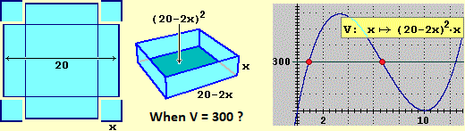
It is necessary to consolidate the concept of domain of a function, focusing that when modeling a problematic situation it is necessary to consider only the intervals in which the quantities represented by the variables can vary
(as in the case of the V function considered just above, in which it is necessary to restrict to
− the general elements necessary to study, at a first level, the functions at an input and an output and to solve equations, without and with parameters, must be provided;
− it must be mentioned and tried the use of symbolic calculation software, even the one incorporated in WolframAlpha;
the reason is, above all, to reduce (in the pupils' mind) the importance of the calculus aspects:
being good and quick to do the calculations is neither necessary nor sufficient to be "good" in mathematics.
To allow the first statistical elaborations and the realization of the first function graphs it is necessary to introduce the concept of interval almost immediately.
It is also necessary to introduce the symbol "∞" and the adjectives "open", "closed" and "limited".
The other different meanings of the term "infinite" (related to the cardinality of the sets) should be introduced later.
A reflection on the setting of geometric teaching in secondary school is to be addressed starting from some general consideration on geometric teaching, which we can entrust to this "digression", fantastic but very concrete, on the concept of angle.
Here various reflections are presented on the inopportunity of an axiomatic approach to the teaching of geometry. This was focused only at the end of the nineteenth century, especially with the aim of focusing on the different geometries that could be defined by changing some axioms. The so-called "Euclid's Elements" (not to be confused with "Euclidean geometry"), significant in the history of thought, certainly do not have the characteristics of what, in mathematics, is an axiomatic presentation: HERE is highlighted as well as the demonstrations of Euclid's first "theorems" are not acceptable.
The objectives that it would be important to privilege in the initial checks and in the recovery activity in the first biennium (at the beginning of the first form or before addressing specific topics) should be more those of "cognitive attitude" and ability to "operate" consciously with the basic knowledge to solve problems. For example:
(a) knowing how to use measuring instruments (ruler, protractor, graduated cylinder, balance, …) to determine extensions (directly or by measuring other physical quantities with which proportionality bonds exist), knowing how to calculate the area of some "strange" figure by using checks or by triangulation, knowing how to compare (with the naked eye) the amplitude of drawn angles (regardless of the size of the segments with which the sides were represented), knowing how to associate the corresponding precision with a measurement, having an idea that the accuracy of direct measurements affects the precision of indirect measurements, … rather than knowing how to recite formulas (direct and inverse) for the calculation of areas of standard figures, being trained to solve stereotyped problems with cones superimposed on cubes, …;
(b) knowing how to use drawing tools (drawing perpendiculars and parallels lines using square and ruler, ...), knowing how to organize the "worksheet" (from the problem of choosing the units on the axes to the problem of where and which figures to draw first to obtain a certain composed figure), knowing how to schematize concrete situations with abstract figures, knowing how to pass from a verbal description of a figure to its drawing and vice versa, … rather than repeating definitions and being able to easily identify figures or elements of figures arranged in "standard" ways;
(c) knowing how to build/interpret scale reproductions (using equations, not with the notorious ad hoc rules for proportions), knowing how to calculate inaccessible distances using similarities, knowing how to associate shadows with objects and other transformed figures to the original ones, … rather than knowing the terms "affine transformations"," homotheties", …
(d) having reflected (not generically) on the differences between common language and specialized languages, having carried out (in simple, but not trivial) contexts some experimentation-conjecture-verification-demonstration activities, being familiar with leading back a problem to other problems (leading back geometric problems to other geometric problems – some of the activities considered in (a) are examples in this sense – creating or interpreting graphic representations of relations between quantities, geometrically visualizing algebraic properties, ...), ... rather than having learned to repeat things like "the point is the geometric entity without dimensions", "we must not speak of equal triangles but congruent triangles because in mathematics two objects are equal only if they are the same", ...
(e) having started the cooperation of the "direct" tools for drawing (ruler, square, protractor, compass, ...) and the use of computer (to create both "freehand" and "geometric" designs), highlighting, operationally, the different techniques and different ideas to use than using non-IT devices.
To exemplify the highest levels of formalization and linguistic precision, of generalization, of "internal" reflection, ... to which we must aim in the initial two years, we can mention:
(a) the use of coordinates not only to graphically represent data and functions but as a way of doing geometry,
(b) Pythagoras' theorem not only for solving problems but also as a cornerstone of Euclidean metric,
(c) the geometric transformations also presented analytically and focusing (operationally) on the concept of "invariant".
Not many concepts and properties that pupils have to understand and internalize (not by learning definitions or demonstrations by heart), essentially related to triangles and circles.
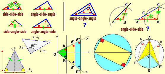
Although an axiomatic definition of the Euclidean plane (or space) is not feasible, we must take into account that it is necessary, in upper secondary school, to give a mathematical presentation, not only experimental (in the "physical" sense of the term), of geometry, both to provide a more explicit and precise view of the nature of mathematics, both to better frame the meaning of the proofs.
| The sum of the angles highlighted in the figure on the left is 360�. What is its value in the case of the figure on the right? Does it have the same value in the case of other similarly intertwined polygons, with the same number of sides? Why? | 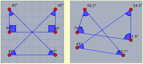 |
| (see) |
On the other hand, a setting should be found which, compared to the traditional one, better highlights the "detachment" compared to intuitive geometry; it is a detachment that is not only linked to the focus of the role of demonstrations, but to a new conceptualization of the "mathematical space". In this sense, a too narrow reference to the space of "physics" seems unsatisfactory and, above all, in the face of the enormous developments that mathematics has had and the many forms through which mathematics has spread in the professions and in the life of all days, an extended and "isolated" treatment of Euclidean geometry seems counterproductive.
Even within the purely mathematical treatment it is necessary to get out of the shell of Euclidean geometry, for example by mentioning the existence of different ways to evaluate distances, such as the simple case of Manhattan distance (equal to the sum of the absolute variations of the coordinates), calculable to by hand or with a simple online program, like this (in the case shown below, the Manhattan distance between (1,3) and (3,5) is 2+2):
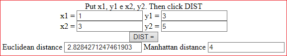
While some geometric concepts are to be introduced analytically:
referring to the plane: • point as a pair of real numbers, • figure as a set of points, • translation as a particular 2 input and 2 output numeric function, • distance as a appropriate 4 input 1 output numeric function, • direction as an element of the range [0°,360°), …
to introduce other concepts and face problems and demonstrations it is necessary to proceed sometimes analytically, sometimes synthetically (for example a half-line, instead of analytically, by means of an equation+inequation system, can be described as the set of points where a given point can be transformed by translations of fixed direction).
These are introductions that abstract and generalize "physical" concepts (from positions on lines and surfaces marked with measuring instruments to points such as n-tuples of numbers, from directions marked by a protractor to the association of an interval [a,b) - the interval [0,2π) - at the points of the circle x²+y² = 1, …), to be addressed after carrying out reflections and operating activities (with drawing and measuring instruments) in "concrete" situations.
And then, the dynamic geometry software can favor these intertwining and abstractions (see the previous and the following example), which can also be developed by relying on animated gifs, such as these.
| How much is the sum of the amplitudes of the opposite corners of a quadrilateral inscribed in a circle? |
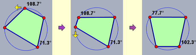 |
| (see) |
The circle, as it is the easiest and most "significant" geometric place, is a geometric concept that must be introduced among the first and on it rests the introduction of various other concepts (direction, trigonometric functions, …). The trigonometric functions (also the tangent function) must be introduced early and not only for convex angles (a choice that would be difficult to reconcile with the introduction of rotations, with references to extra-mathematical applications, with the use of calculation means, …). The directions (and the measures of angles) and the measures of areas and lengths can only be introduced through an unformalized use of the concept of limit (not with considerations on "contiguous classes" or similar, difficult to rigorously formalize), in accordance with what was previously observed on the introduction of real numbers).
| The calculation of the arc AP length (see) | ||
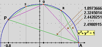 | 1) consider points A and P 2) write the length of the sthe broken line that joins these points 3) add to each pair of successive points the circle with abscissa in the middle of their abscissa 4) go back to point 2 |
|
Polygons can be defined as unions of triangles, so as to also include polygons with concavity and "self-intersecting" polygons, and in order to avoid non-trivial issues connected with the subdivision of the plane by closed lines (see). Conics can be introduced starting from the circle and from the graphs of the functions x → ax² and x → a/x, using plane movements. Other geometric transformations can also be introduced, intertwining synthetic and analytical characterizations in an appropriate way.
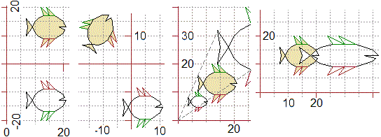 |
Next to the Euclidean plane, other mathematical spaces can be presented immediately, without in-depth analysis: finished spaces, spaces with other metrics, spaces with other dimensions, … to better focus on the "abstract" nature (and on the connected capability to model situations) of the geometric concepts. As already observed, the differences between intuitive arguments and demonstrations must be gradually brought into focus, and the conflicts between mathematical terminology and common language highlighted (the different meanings of angle, direction, distance, curve, ...).
In the following years the topic of three-dimensional geometry will be deepened. Anyway, as flat geometry topics are introduced, it is appropriate to sketch their development in space, taking up and making a first probing of topics that should already have been addressed in the lower secondary school (see). For example, it will be necessary to mention how with the coordinates it is possible to represent points of the space (not only of the plane), how to read a map with the level curves represented, how three-dimensional objects can be distinguished on the basis of symmetries:
|
|
|
|
The last image recalls a geometric theme mentioned in other paragraphs (those on circular functions, inverse proportionality, mathematical structures): the theme of translations and vectors, which, in schools where the study of physics is already foreseen in the first two years, it must be addressed, at a first level, also in the three-dimensional case.
The following images recall other aspects that can be addressed, with links to other disciplines: the question of cartographic reproductions (A preserves the areas, B preserves the intersection angles, C the rectilinear trajectories),
the problem of movement on a non-flat surface (the ant that walks starting along an "equator" of the ball keeping perpendicular to the "meridians" remains on the equator, the one that starts from another parallel never retraces its steps;
an ant that walks on a plastic cone without turning arrives on the lower edge,
just like we, walking in the mountains, if we do not push more with the below foot we go down to a lower level).
 |
|
|
|
|
These concepts will have to be resumed and deepened in the following classes, with a view to a "spiral" recovery of the topics, and taking into account that for the same topics different levels of probing can be envisaged: it is not a question of making "anticipations", but to use, in appropriate ways, terminologies and concepts that find natural intertwining with other concepts and to lay the foundations for the construction of subsequent levels of formalization. We think this aspect is fundamental, both to give a correct and "lively" image of mathematics, and not to favor mental stiffenings that identify concepts with particular definitions, particular calculation procedures, … and classify them into areas (geometry, algebra, analysis, probability, …) not communicating with each other.
A more in-depth discussion of the setting of geometric teaching, with a quick history of geometry itself (and various exercises for teachers), can be found here (in Italian).
We mentioned, in the previous paragraph, the opportunity to introduce, at a first level, the circular functions, indispensable for dealing with both the first geometric transformations and the first scientific area activities foreseen in the other disciplines (in which vectors, slopes, … intervene).
slope = 5/10 = 50% 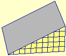 |
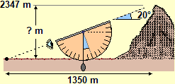 slope = ? / 1350 slope = tan(20*gradi) ? = tan(20*degrees)*1350 = 491 |
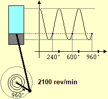 |
The first of the previous figures recalls the presence of circular functions when evaluating the slope of a road, or a graph; the second, their role in assessing the height of a mountain with the vertical protractor (by resuming things that can be tackled in basic school, and starting to use calculator and software appropriately). The third figure operationally displays the graph of a periodic function whose trend can be easily understood (and of which the analytical expression can only be studied in the following classes).
As already mentioned for other topics, the concepts must be gradually introduced over the years, intertwining naturally with other themes. In this case, the study of circular functions must be resumed in all subsequent years of high school.
Obviously, the introduction of circular functions precedes the "study" (not "use") of polynomial functions, which will require more advanced technical and conceptual knowledge.
It is worth noting that circular functions should not be introduced only for convex corners; this could have made sense in the past (up to the mid-twentieth century), when calculators did not exist and when trigonometry was mainly studied for topographical problems.
The function of inverse proportionality is one of the first that is studied in compulsory school, it is of fundamental importance in all mathematics and in all its applications, and its recovery must obviously precede the introduction of polynomial functions. Certainly in the lower secondary school situations such as those illustrated in the first two figures were addressed, in which it is highlighted that, with the same effect, the force exerted and the length of the trajectory along which it is exercised are inversely proportional. Also the idea of what part of a win to the football pools is up to each of the winners according to the number of them or (see the graph on the right) of how much a photocopy costs on average in a month (CU - unit cost) made with a copier rented monthly (given the cost of the rental and given the incorporated cost, CI, of the raw materials - paper and toner) as a function of the number of photocopies made, they are examples of inverse proportionality functions that may have been faced.
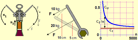
In the first two years of upper secondary school, starting from examples of this type, it is necessary to study the abstract functions
e
We have already observed that a constructivist approach to real numbers is indispensable if we want to use square roots (if not, who tells me that there is the square root of 2?) or if we want to consider segments of "exact" length (like a long segment 5.010010001…), that is it an approach in which
• the real numbers are presented as appropriate sequences of characters (digits, "." and "–"), with a suitable "equality" relationship (3.7999… = 3.8000…, etc.),
• operations on limited decimal numbers are defined algorithmically,
• and are then extended to real numbers through the concepts of approximation and, without formalizations, of limit and of continuous function (e.g. to obtain the result of x·y with a certain precision, it is sufficient to operate on indeterminacy intervals for x and for y sufficiently little ones).
In turn, the reflections (both deepenig and synthesis) on the resolution (graphic, numerical and symbolic) of the equations must not aim to develop technical specifications, as methods based on the more or less formalized use of some concepts general: inverse function, injection function and continuity.
At this point, already in the first two years, a first formalization of the concept of continuity can be given: let F be a function defined in an interval [a, b]; if as the inputs are denser also the outputs are denser, then F is said to be continuous on [a, b]. Furthermore, if F is a function defined in any set I of real numbers, it will be said that F is continuous on I if it is such in every interval [a, b] contained in I (for example
The following figure (in which we plot the graph for an increasing number of points) makes us understand that the function
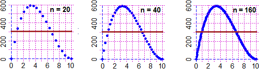 |
The choice of introducing continuity (of real functions of real variable) on intervals, not at points, is the standard one in the field of constructive mathematics and is made in various calculus manuals. In addition to facilitating the introduction of integration (otherwise it should be shown that pointwise continuity implies that on intervals, which is not easy, and over which textbooks often pass, resorting to incorrect demonstrations of the integrability of continuous functions), has two advantages:
• it is closer to the "intuitive" concept of continuity (which is not "punctual") and is suitable for all the developments that can be tackled in upper secondary school;
• it corresponds to the concept of "tabulable function", that is a function F that can be (graphically or tabularly) represented with a calculator: however we fix Δy we can find N such that, dividing [a,b] in N equal intervals,
This is a typical example of an educational solution that could overcome some of the conceptual difficulties that pupils encounter in dealing with the topic in question.
In the context of the study of learning processes, these difficulties are often linked to the presence of some "epistemological obstacles", which one try to identify both with "theoretical" reflections and through appropriate experimentation activities.
Sometimes, however, these researches refer to a presentation of a certain mathematical concept (to understand each other: the continuity defined punctually, the primitive geometric entities presented axiomatically, ...) which is taken as "absolute", without worrying about the possibility of various presentations (often with sensational misunderstandings of the chosen mathematical presentations: think of the conceptual confusions on arithmetic and geometry present in Piaget's works and, above all, of his followers).
If you want to deepen the topic see here.
Systems of equations. Inequations
The resolution of systems can be introduced naturally in connection with geometric issues: this is the most effective way to start (and develop in a general, and not mechanical) way the main topics and the main attentions related to this area of mathematics.The resolution of systems can be introduced naturally in connection with geometric issues: this is the most effective way to start (and develop in a general, and not mechanical) way the main topics and the main attentions related to this area of mathematics.
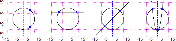 |
x2+y2=100 & x=6, x2+y2=100 & y=6, x2+y2=100 & y=x, x2+y2=100 & y=x2−12
But, obviously, many situations faced since basic school should have already started this topic, both "geometrically" and, above all, in relation to common problematic situations, such as the following:
 Luigi - 30 € |
 Maria - 44 € |
And the use of dynamic geometry software, which "automatically" identifies the intersection points, for example between a segment and a circle, can pose the problem: how does the program determine its coordinates (and then trace them)?
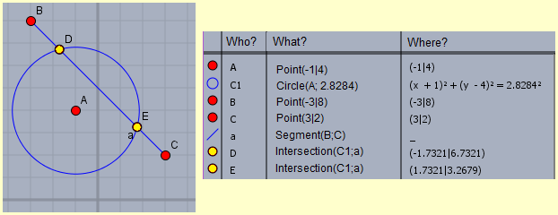 |
After focusing on the topic in general, we can dwell on linear systems, highlighting their characteristics in relation to the number of solutions. The introduction of strange (and almost never efficient) tricks, such as the "Cramer rule", should be carefully avoided.
Instead, it is good to educate students on some essential aspects: • in the absence of parameters, if the unknown is a pair of variables, resort to graphic methods to estimate the solutions, • before starting to do manipulations, see if there are ways easier to find the solutions directly, • check the solutions found, …
The reflection on the differences with respect to the other systems of equations can also be highlighted by reflecting on the possibility of solving linear systems in a "mechanical" way, using software. Here, for example, the use of a simple script for a system
of two equations:
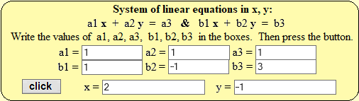
and of this for a system of three equations (and of this for a system of four equations):
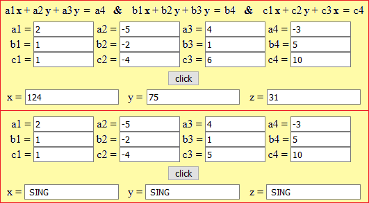
Only in the final classes of high school, and only in some types of schools, it will be possible to dwell on the concept of determinant (see) and to frame the problem in the context of matrix calculus.
As already observed for the previous items, before doing exercises without a reference context, it is good to consider problematic situations, such as the one shown below on the left: from the graphs of costs and revenues relating to a particular production, obtain when there is a situation of balance, or when the gain is "positive". This is also a simple example of solving an inequation. Focusing, with simple but significant examples, the concepts and their use, is an essential aspect, much more important than that of preparing experienced users of some formula or mechanical procedure (experienced only as long as they remember it!).
|
|
As has been said for systems, the concept of inequality must be considered in a general way, taking into account the way it presents itself in many concrete situations (for which x
We have seen that one of the first concepts to be resumed and deepened is that of function, in the form of both an algorithm and a table and a graph, and that the reference to this concept comes into play in the definition of terms and, therefore, of formulas.
We have also seen that the reflections (both of analysis and synthesis) on the resolution (graphical, numerical and symbolic) of equations, systems and inequations should be directed not so much at the development of technical specifications, as at the identification of methods based on the use of some general concepts (inverse function, injection, continuity, logical connectives,
From the beginning it is good to examine various types of functions (and equations), even if only a few will be studied more deeply (without this more general framework, the characteristics of the latter could not be highlighted by contrast). We observed that both the introduction of ad hoc techniques for issues that can be addressed with more general methods, and the development on particular cases of aspects which, without expenditure and with greater significance, can be seen in more general contexts, should be avoided.
With this premise, which in some way takes up what has been observed on the concepts of function and solution of an equation, we want to underline the importance of starting the study of polynomial equations only later, towards the end of the 2nd year.
On the other hand, these, and more generally the polynomials, are introduced in funny and incorrect ways in many textbooks (see, for example, what has been observed here).
Unfortunately, the ways in which polynomials are often introduced in upper secondary school leaves a lasting mark, even in those who continue their studies, both among those who enroll in scientific faculties (see the results of this exercise), both among those who graduate in them (see the results of this other exercise).
Here, in our opinion, briefly, the arguments relating to the polynomial functions that (between the end of the second year and the beginning of the third) should be addressed:
• the polynomial functions F have the characteristic of having a graph trend and the value of the solutions of
• polynomial functions are all continuous on R;
• between the polynomials there is an operation of division with remainder, which has various analogies with that between integers;
• the factor theorem (also known as Ruffini's "remainder theorem"):
P(x) as a factor (x−k) if
• a polynomial equation of degree n has at most n solutions;
• the solution of a 2nd degree polynomial equation can be interpreted as the search for intersections with the x axis of a parabola whose coordinates depend on the coefficients of the equation itself;
• it is useful to memorize the factorization of some polynomials into polynomials of a lower degree.
After focusing on the theorem of the rest and the link between the degree of a polynomial equation and the maximum number of solutions, one can resort (as we have seen considering the equations) to software to graphically represent functions and other software (for example WolframAlpha) to solve any polynomial equation: there is no need to focus on techniques for solving polynomial equations of a degree higher than the second, if not those that can be studied using simple factorizations. An example:
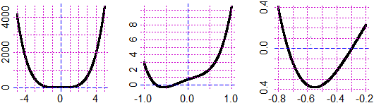 solve 7*x^4+sqrt(3)*x^3-x^2+2*x+2/3 for x real -0.29422093345889… -0.732580963760389… |
Then, at the end of high school, one will see the importance of polynomial functions as they allow us to approximate, around particular points, many other types of functions, more difficult to handle (approximations with first or second degree polynomials and, in some types of schools, Taylor's polynomials and series).
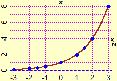 |
On the side the graph of the function |
|
21.5 = 215/10 = 23/2 = (23)1/2 = √8 = 2.82842… 2−1.5 = 2−3/2 = 1/23/2 = 1/√8 = 0.353553… | |
|
With a means of calculation I obtain values also for other exponents; for 2π with WolframAlpha I have for example: 8.82497782707628762385642960420800158170441081527148… Let's remember how the calculation could be done in these cases: |
| π = 3.1415926535897932384626433832795028841971693993751… | ||
| 23 = 8 | ≤ 2π ≤ | 24 = 16 |
| 23.1 = 10√(231) = 8.5741877002… | ≤ 2π ≤ | 23.2 = 10√(232) = 9.1895868399… |
| 23.14 = 50√(2157) = 8.8152409270… | ≤ 2π ≤ | 23.15 = 20√(263) = 8.8765557765… |
| ... | ... | ... |
| 23.141592 = 8.8249738290… | ≤ 2π ≤ | 23.141593 = 8.8249799460… |
| ... | ... | ... |
What we have seen now is the way in which the function x → 2x: for rational x it is defined in the way illustrated at the beginning of this entry, in other cases it is defined as we have now seen, so as to be continuous, i.e. so that when the inputs are thickened, the outputs also thicken.
If there is no need to introduce the exponential function in the first two years, it can be introduced, similarly, to the third year. In textbooks, the exponential function is often used brutally, without having defined it except for whole inputs!
In discussing the concept of real number, we saw how, in the first two years, we can deal with a first reflection on the "algebraic" differences of the different numerical structures, intended as substructures of R.
Once other mathematical objects (functions, sets, vectors, geometric transformations, ...) and ways of working with them have been introduced, some of the various structural analogies (and differences) between numbers and these objects can be briefly presented in the second or third year.
The goal is not to add other notions, but to focus on links, similarities and diversity, both to contribute to the formation of an idea of the more or less explicit links that exist between the various areas of mathematics, and to to encourage the transfert (and unification) by students of ideas, methods, concepts between different sectors.
It is a matter of creating a synthesis of aspects that should have been highlighted gradually in teaching, with different levels of depth depending on the type of school and class.
The mathematical objects considered are not entirely new compared to previous school levels; what is new is to synthesize and unify them by referring to more general ideas.
| g+f f+g f(g(.)) g(f(.)) "ca"+"sa" "sa"+"ca" not(P and Q) (not P) or (not Q) | ||
| I translate by the vector (2,1) and rotate around 0 by -90° I rotate around 0 by -90° and translate by the vector (2,1) |
| |
Some mention should be made of "modern" algebra, which specifically addresses these connections. The goal is not to make it a specific object of study (which can be tackled successively by those who continue their studies in the scientific field), but to contribute to the formation of a unitary idea of mathematics. Some of these objectives may be taken up and deepened in the last years of high school.
In schools with a more professionalizing approach, these aspects will obviously be addressed in a more operational way.
| How many poker hands are possible? | y(0) = 1, y(n+1) = (y(n) + A/y(n)) / 2, y(n) → ? |
|
A biologist must do an experiment on 60 mice, chosen from the 100 available. In how many ways can he make the choice? |
Check by the computer that for a positive integer n 1³ + 2³ + 3³ +…+ n³ = (n·(n+1) / 2)² (see) |
 | (script) |
An important concept to focus (also for the various applications that it will find in the following classes) is that of definition by recursion, that is, of the definition of a function F (or of other mathematical objects) by means of equalities in which F appears both at first than to second member. Among the functions we include the sequences, which are nothing more than functions having as input the natural numbers (all or those starting from 1 or from another natural number), which can be indicated with the usual functional notation (a(1), a(2), a(3), …, as is done in many mathematical analysis manuals), or by enclosing the input in square brackets (a[1], a[2], a[3], …) or using the expressions a1, a2, a3, …
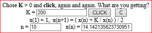 | (click here) |
Recursive definitions are also used to characterize different concepts of combinatorial calculus.
The latter is an area of mathematics rich in applications, with many connections with other sectors, pure and not (analysis, algebra, probability calculation, ...), which requires good, but simple, ability to model various types of phenomena, and which cannot and should not be trivialized, as unfortunately almost always happens, in the solution of some battery of stereotyped exercises.
It is essential not to make students learn formulas by heart, but to teach them to derive and adapt them. Most combinatorial problems cannot be addressed using directly some standardized solution procedure, but by resorting to ad hoc, simple but significant forms of reasoning: understanding (and the mathematical representation, in different forms, which may vary according to the "tastes" of people) of the problem to be addressed is fundamental.
Addressing the descriptive statistics, the basic concepts and techniques for the representation and study of random variables should already have been introduced. By addressing the calculus of probability the transition is made to the case in which "forecasts" are made, on the basis of statistical considerations, beliefs or information of various kinds. Combinatorics, now considered, offers some tools to make these predictions, in some particular cases.
|
Probability should have already been addressed in previous schools, but often this does not happen, or it happens in "harmful" ways:
think of the many books in which "definition" is defined as the ratio of |
|
Of the concept of probability it is necessary to specify the rules to which it must submit, making it clear that the choice of the probability values to be assigned does not depend, in the first instance, on mathematical considerations, but on experiments, ideas, assumptions, ... in which mathematics has no leading role. In practice it is an axiomatic definition (the one recalled in the following figure, in which A1, A2, A3, … are incompatible events), like various other definitions that pupils have encountered in their studies, even if they were not called in this way (much of the arithmetic, for example, is learned "axiomatically"; also the concept of distance, Euclidean or Manhattan, is defined in this way). This is the first context in which it is clear and significant to explain this aspect: it is "obvious" that if I believe that with the probability of 50% Inter will beat Milan and that at 20% the two teams will draw, for me at 100% - (50% + 20%) = 30% Milan will beat Inter. "Cases/cases" have nothing to do with it, only the properties referred to in the following figure are involved, which are none other than the properties already seen for the percentage frequencies, the same that are used to trace areograms, histograms, boxplots, .…!
 |
In addition to situations, such as that of the previous example (Inter-Milan), in which the probabilistic assessments are subjective, or that of the unfair dice, in which they can be made after assigning a probability of exit to the various faces after the experiments, there are also situations where the outputs are infinite, as in the following example. That's why the "..." in the figure above.
|
I throw a balanced coin N times until I get "heads". Sometimes N = 1 is enough, sometimes N = 2, sometimes N = 3, ..., but an innumerable number of attempts may be necessary. What is the probability that N = 1 is enough? That N = 2 enough? ... |
There are, moreover, simple situations of which it is not easy to find the solution theoretically, or where you want to check it to be sure. In these cases it can be useful to use the computer, to simulate the phenomenon with the random number generator and study it with statistical tools. An example, to clarify this aspect:
| What is the probability that throwing two balanced dice the difference of the exits is 1? Experimentally: Event = function() abs( RUNIF(1, 1,6)-RUNIF(1, 1,6) ) == 1
PR = function(n) {f=0; for (i in 1:n) f = f + ifelse(Event(),1,0); f/n*100}
PR(1e4); PR(1e5); PR(1e6)
# 28.17 27.607 27.7118Theoretically:the good outputs are 12, 23, 34, 45, 56, 65, 54, 43, 32, 21, e 10/36 = 5/18 = 27.777… |
As we have seen, the tools that intervene to mathematize situations of uncertainty are largely the same as those used in other areas of mathematics. Tree graphs and percentage breakdown tables are particularly useful for tackling another concept that must be focused on in the first two years: that of dependence/independence of events and random variables:
|
What is the probability that, when I cut the cards twice, I always get a denier card? |
 |
What is the probability that, when I extract two cards from a pack, I always get a denier card? |
 |
Many of the examples that can be faced refer to the game, partly because of the very nature of the probabilistic concepts, partly because they are more easily modeled situations, in which it is more convenient to extract the significant aspects. But it is also good to refer to non-gaming contexts, for example to situations in which, based on probabilistic assessments, choices must be made in a productive activity or in a judicial context, or where assessments of a biological or health nature must be made. Just think of genetics or the context highlighted by the following example, or the one highlighted by this other.
|
A certain health test to evaluate the presence (positive outcome) or absence (negative
The probability is 0.95% / 5.90% = 16%, much less than 95%, as might have been thought. | ||||||||||||||||||||||||||||||||||||||||||||||||||||||
The fact that probabilistic tools are to be used (and whose outcomes are to be interpreted) in contexts that are not purely mathematical is perhaps the reason why they are often overlooked by teachers or developed in completely incorrect ways. On the contrary, it is essential, from an educational point of view, to tackle this subject, also trying to highlight the difficulties and errors that pupils can commit by tackling probabilistic issues. This is a decisive aspect for this area of mathematics, for the issues addressed above, and to encourage the development of attentions towards the nonsense that various mass media often propose by referring to probabilistic evaluations.
This area of mathematics is perhaps the one that, compared to the others to be addressed in the first two years, requires a more structured development, also opening up to a more organic way of carrying out the themes that should characterize the following years. In the second two years the areas of statistics and probability will find a stronger intertwining, when the central limit theorem has been focused. However, the idea that, in a statistical experiment, as the number of tests increases, the ratio between the number of favorable exits and the total of exits tends to stabilize on probability constitutes some form of anticipation. Here you can find cultural, didactic and technical considerations that deepen some aspects. Here you can find a short history of probability.
The random number generator (which we have discussed several times) is often called pseudo-random number generator because the numbers are produced by a program that generates them according to a certain algorithm with a distribution that is "practically" uniform. By choosing a particular value (called "seed") you can cause a particular sequence to be generated. For further information see HERE. It can also be used to encode and decode ("secretly") texts; see HERE.
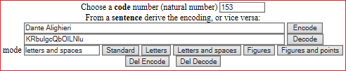
Using the R software a teacher can easily reorder the order numbers of the quizzes in a classwork. The teacher chooses the seed, for example 120, and rearranges the questions (for example 15) for his 30 pupils with the following commands, preceded by source("http://macosa.dima.unige.it/rR"):
| set.seed(120+1); sample(15) | getting: | 4 12 14 7 15 9 1 3 8 5 11 10 2 13 6 |
| set.seed(120+2); sample(15) | 8 9 10 12 7 14 2 4 3 13 11 15 1 6 5 | |
| ... | ||
| set.seed(120+30); sample(15) | 3 14 15 1 13 4 5 7 8 9 11 12 2 10 6 | |
| or, if the questions are indicated with letters: | ||
| set.seed(120+1); SAMPLE(15) | D L N G O I A C H E K J B M F | |
| set.seed(120+2); SAMPLE(15) | H I J L G N B D C M K O A F E | |
| ... | ||
| set.seed(120+30); SAMPLE(15) | C N O A M D E G H I K L B J F | |
Or, if the questions are closed-ended, with e.g. with 5 and 4 answers, you can reorder the possible answers:
set.seed(120+1); sample(5); set.seed(120+1); sample(4) 4 5 3 2 1 4 3 2 1
set.seed(120+2); sample(5); set.seed(120+2); sample(4) 1 2 3 5 4 4 1 2 3
...
Alternatively, you can use this simple script.
Educational differentiations
What we have indicated are the topics that could be addressed in the first two years of high school, taking into account that the level of deepening can be different depending on the type of school, and also on the characteristics of the individual classes.
In the first year there are pupils with different "abilities", not easy to explore: often the school obscures or overestimates the skills and potential of the various pupils, while the first weeks of school should be aimed at investigating, not fiscally, with various activities, their cognitive styles, their knowledge, their misconceptions, … At the beginning of the second year, the possible arrival of new pupils should be addressed with similar attention.
In many paragraphs we have seen how the software can be used to facilitate the didactic management of many contents, allowing to face the same themes with different levels of technical deepening in different school realities.
And, beyond the use of software, it is necessary to identify the essential mathematical contents and methods to be addressed in each context, interweaving them with the other disciplinay areas, in a different way, for example, in a school with an artistic orientation compared to one with a scientific or technical or classic or commercial address.
And it is necessary that, in the same class, the topics are addressed so that everyone can follow the "thread of the discourse" and understand the essential aspects of the mathematical concepts introduced, taking into account that, in the spiral resumption of the same that must characterize the teaching in subsequent years, pupils will be able to consolidate their mastery at different times.
And it must be taken into account that the continuous renewal of mathematics, of its uses, of its interactions with other disciplines, of the available technologies, of the opportunities offered by the network require that many of the contents and techniques, which have become obsolete, are gradually reduced or " thrown overboard "to give space to new contents and new techniques, and to attitudes that allow to find, select and use what the new media propose.
Mathematics is alive.