On some mathematical concepts / themes to be faced in the last years of upper secondary school
("interwoven" within teaching units)
[primary - A primary - B lower secondary upper secondary - A upper secondary - B school]
The concept of model
Real (and complex) numbers
Non decimal numbering bases
The concept of limit
Continuity, integration, differentiation, antidifferentiation
Exponentiation and logarithm
Space
Statistics and theory of probability
Relationships between two random variables
Insights on mathematical analysis
More
Educational differentiations, and final considerations
In the last years of high school, in addition to in-depth themes already present in the previous school levels, new themes are being launched (differential and integral calculus, but not only).
They are presented articulated by thematic areas but, as it is clarified, in the didactic paths the different mathematical concepts must intertwine with each other and with the other disciplines.
Some of the themes presented in the part relating to the early years of of upper secondary school, although not mentioned here, must be taken up and developed in these final years.
In the last paragraph there are indications on the possible diversification of educational development in the various types of schools.
Examples of the use of animated gifs, useful for introducing various topics in a more intuitive way at different school levels, are present HERE.
Mathematics can be called the science of models. The concept of model must therefore play a central role in its teaching from the first levels.
For further deepenings on these aspects, we refer to the document relating to the first years of high school.
Mastering the decimal representation of numbers should be one of the objectives of teaching in lower secondary school.
It is essential that didactic activities have been set up at the beginning of high school that have allowed to verify this mastery and possibly to start activities that have consolidated it.
A similar attitude should be held for any new pupils who got into the last high school classes.
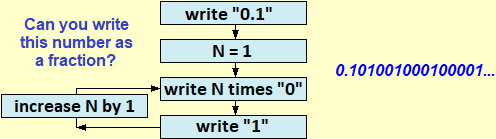
We remind only the following "summary" image and some considerations.
For a correct and meaningful introduction of numbers it is appropriate to choose a constructivist approach; In short:
– real numbers as appropriate sequences of characters (digits, "." and "−"), with an appropriate "equality" relationship (3.7999…=3.8000…, etc.),
– algorithmic definition of operations on limited decimal numbers,
– extension of these to real numbers through the concepts of approximation and (without formalization) of limit/continuous function (e.g. to obtain the result of x·y with a certain precision, it is sufficient to operate on sufficiently small uncertainty intervals for x and for y).
Natural numbers, integers, periodic numbers, limited decimal numbers and those limited in other bases are studied as particular subsets of R which are closed under some operations.
Obviously, it is not appropriate to introduce the real numbers axiomatically, nor to present the construction of the various numerical sets starting from N:
– it would be expensive and difficult to introduce the algebraic-logical-set-theoretic tools to "correctly" carry out the construction (even just the passage) to the integers;
– and, above all, at this level, there are no "didactic" motivations (in a university course of algebra the construction of Q starting from N can instead be an occasion for the application of concepts such as partition, immersion, …) or "cultural" (in a university course on the foundations of mathematics it can instead be significant to construct a model for the axioms of real numbers by set techniques beginning from Peano's arithmetic).
Those now referred to are concepts and methods that must be introduced in previous years and that must be taken up again in recent years, intertwining with issues discussed here talking about continuity, integration, differentiation, antidifferentiation. In high school, it is necessary to mention another concept with which those who carry out a job that has to do with the use of the computer (or with electronic technology) will surely have to do: complex numbers. Let's start with an example.
If with WolframAlpha I solve the polynomial equation 2/3 + 2 x − x2 + √3 x3 + 7 x4 = 0 I get:
solve 2/3 + 2*x - x^2 + sqrt(3)*x^3 + 7*x^4 for x
−0.294221 −0.732581 0.389683−0.53852i 0.389683+0.53852i
To get only the real solutions I have to add:
solve 2/3 + 2*x - x^2 + sqrt(3)*x^3 + 7*x^4 for x real
At this point the question arises as to why these strange numbers are displayed? What are they for?
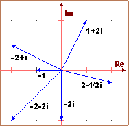
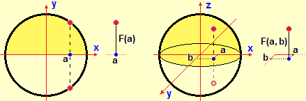
A first answer, which can be faced with all the pupils, is recalled in the first of the following figures:
complex numbers are an alternative way to describe the vectors and points of the plane (for example, the sum of two complex numbers equals the sum of the corresponding vectors).
A second answer, which can also be addressed with all the pupils (if there is time available), is the one recalled by the second figure: with the complex numbers many geometric transformations can be easily described, in this case the one that revolves around
Conformal maps (or trasformations), such as the one represented in the third figure, can also be studied in scientific and technical high schools.
To learn more about these aspects, in a possible worksheet for students, see here (it is in Italian but can be translated via software).
In paragraph 6 of it you will also find some historical reflections on the "strange" origin of complex numbers (as a trick to solve some polynomial equations), which can possibly be addressed in high school.
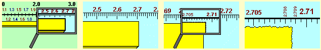
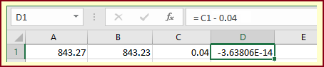
With this calculator if I run 843.27−843.23 and
I try to run them with a spreadsheet. I examine what is obtained in the first case (see the following figure). I seem to get the expected result (0.04) in C1 (where I put "=A1−B1"), but if I make the difference between the result obtained and 0.04 I don't get 0! If I calculated the difference between the two values (0.04−3.63806e-14) I would obtain 0.03999999999996362, a value similar to that obtained with the previous calculator. In the case of spreadsheets (unlike other free, but more reliable applications such as R) it is less easy to explore these facts (it is necessary to extricate oneself in a menu made on purpose to have nice effects but which is not suitable for carrying out non superficial considerations; the financial problems that some banks have encountered using spreadsheets have been various: a small difference, if not seen, multiplied by large numbers, can give rise to very large values).
How come this happens?
Unlike what happens in the usual calculators, which store numbers in decimal form (store single digits in binary form), most computer applications store numeric values (in the registers associated with variables) in binary form.
You can get an idea of how this happens with this simple application.
Here are two particular outputs, for the calculation of the ratio between two integers expressed in decimal and binary form:
|
Division of m by n with m < n (natural numbers in base ten) and result in a base of your choice By clicking [one step] you gradually get the figures of the result m = n = base = remainder = |
|
Division of m by n with m < n (natural numbers in base ten) and result in a base of your choice By clicking [one step] you gradually get the figures of the result m = n = base = remainder = |
The concept of limited number (i.e. number with period 0) depends on the basis of representation. 1/2, which in base ten is 0.5, in base two becomes 0.1; but 1/10, which in base ten becomes 0.1, in base two it becomes the unlimited number 0.00011001100110011… as I cannot express 0.1 as the sum of a finite quantity of fractions taken between 1/2, 1/4, 1/16, 1/32, ... (which, written in base two, become 0.1, 0.01, 0.001, 0.0001, …). At this point it is easy to understand the strange exits considered at the beginning of the paragraph. 843.27 and 843.23 are internally expressed in binary form and approximated, the difference is made between these two numbers in base 2, and the result is displayed in base ten: 0.03999999999996362 is the result, which differs from 0.04 by the decimal value corresponding to the binary digits that have been lost.
The programs considered manage to represent a finite number of numbers. Therefore, they also have a maximum number. With the calculator considered at the beginning of the paragraph the maximum number that I can calculate is 21024 (1024 is equal to 2 to 10, that is, in base 2, to 10000000000); 1.797693e+308 is given as a result; if I increase the exponent by 1, or by 0.00001 the base, an overflow error is signaled to me.
With students of all types of schools, beyond theoretical deepenings, it is necessary to focus, operationally (by making them do calculations, mistakes, comparisons, …), the fact that the means of calculation carry out the calculations not in decimal form and that the numbers that appear displayed are not necessarily the same as those stored internally.
The word "limit" (and words derived from it, such as "limited", "unlimited", …) is used many times in mathematics. For example it is said that:
– the interval [3, ∞) has no upper limit,
– a point that proceeds beyond all limits in a fixed direction describes a half-line,
– an angle is an unlimited figure (i.e. that extends without limitations),
– an unlimited decimal expression continues after the "." with an infinite sequence of digits.
In these cases, as also in many non-mathematical contexts («within certain limits», «speed limit», …), "limit" indicates something that cannot be overcome.
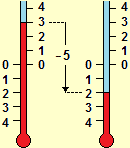
In other situations the limit word is used with a somewhat different meaning:
«after the opening of the parachute he began to brake, and the falling speed gradually stabilized on the limit value of 20 km/h», ….
These are cases in which we are considering a certain process that evolves towards a limit condition; here we use "limit" in the sense of a state that a certain phenomenon tends to assume.
| The figure on the right should clarify the difference between the two uses. If I give a small downward push to a rubber ball immersed in a bucket of water, the ball begins to swing: its center drops to the L1 altitude, then rises to the L2 altitude, then drops a little less, then goes back up, …; ; L1 and L2 are a lower and an upper limit to the position that the center of the ball can assume; as time passes, the oscillations damp and the center of the ball tends to assume the limit position L. | 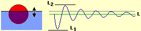 |
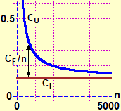 |
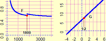
In this paragraph we focus on the second use ("limit" as a state to which a process tends), which is the most frequent one in mathematics, and which more or less explicitly should have already been used many times in the previous classes: • The number 0.101001000100001…, the truncation approximations 2, 2.2, 2.23, 2.236, … of √5, the periodic number 3.777… indicate the "limit" expressions to which these writing processes tend, which we can never complete. • In the case of the rental of a photocopier, the unit cost of a photocopy tends to coincide with the built-in cost of paper and toner since, with the increase in the number of copies made, the fixed costs tend to be amortized (see the graph on the side). • By repeatedly tossing a (balanced) coin the relative frequency with which "head" comes out tends to stabilize at 0.5. |
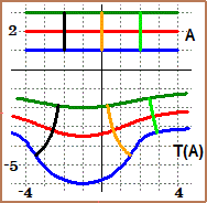
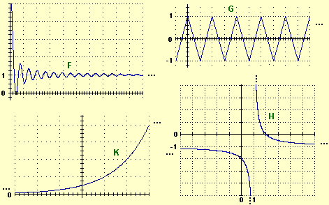
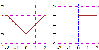
Rather than "formally defining" the concept of limit, the problem of constructing its meaning must be addressed. For example, restricting oneself to the real-valued functions of a real variable, it is necessary to learn to describe, starting from the graphs, particular behaviors of them using the lim symbol:
|
|
|
|
|
|
|
|
The meaning of limit can then be expressed "in words". For example, if the input tends to K and the limit L is finite, I can say: "by bringing the input value closer to K, I can make the output stabilize as close to L as I want"; or, if L is ∞, I can say: "by bringing the input value closer to K I can make the output greater than whatever it has set". And it can be made that the students (now or when we will tackle the link between statistics and probability - see) reflect upon the fact that, in the case of the coin toss, the relative frequency with which "head" comes out tends to stabilize near 0.5, but not with "certainty".
|
It is necessary to focus on some important aspects, such as the following, which refers to the two figures on the side, in which the red dots indicate points that do not belong to the graphs. |
 |
It is then easy to focus, through examples and "graphic" reasoning,
that the passage to the limit preserves sums, products, quotients and the order relations ≥ and ≤ .
In the case shown below on the left we have that the limit of
With a few simple graphic examples we can understand how to extend the properties considered above to cases where the limits are infinite.
For example if
In high schools it can be seen how the properties relating to the transition to the limit of (for example) a sum of functions can be translated into more formal ("ε-δ") explanations. But this can only be done to give pupils an idea of how the reasoning could be translated into more rigorous procedures, not as arguments to explain these properties.
The limits of the sequences must be treated as limits of functions as the input approaches infinity; they should not be studied as a separate topic!
Continuity, integration, differentiation, antidifferentiation
In the document relating to the first years of high school we saw how, having consolidated the concept of function (see), it is appropriate to give a first formal arrangement to the concept of continuity already in these school years
(see):
let F be a function defined in an interval [a, b]; if as the inputs are denser also the outputs are denser, then F is said to be continuous on [a, b]. Furthermore, if F is a function defined in any set I of real numbers, it will be said that F is continuous on I if it is such in every interval [a, b] contained in I (for example
For example, a function such as
 |
We recall that this choice of introducing continuity (of real functions of real variable) on intervals, not at points, has several advantages:
• it is closer to the "intuitive" concept of continuity (which is not "punctual") and is suitable for all the developments that can be tackled in upper secondary school;
• it corresponds to the concept of "tabulable function", that is a function that can be (graphically or tabularly) represented with a calculator: however we fix Δy we can find N such that, dividing [a,b] in N equal intervals,
• it facilitates the introduction of integration (otherwise it should be proved that punctual continuity implies that one on intervals, proof which is not easy, and over which textbooks often skip).
Having introduced in previous years how to calculate the area of any polygon (for example as a union of triangles or as a difference of areas of trapezoids) starting from the coordinates of the vertices, it is now easy to introduce the concept of definite integration.
The area between the graph of a function f and the x axis, for x that varies between a and b, can be approximated with the area
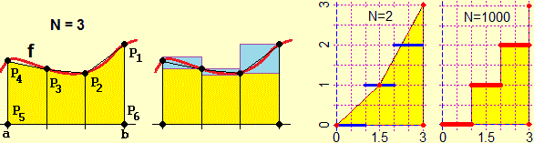
The figure above right illustrates the case of a "piecewise continuous" function, ie defined on an interval which is the union of intervals on which the function is continuous and limited. Also in these cases the procedure stabilizes on a number, which we take as the value of the area underlying the graph.
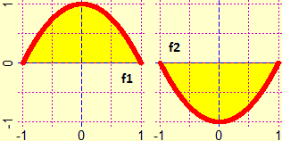 |
On the side, the graphs of f1 and f2 are represented, as the abscissas vary between −1 and 1.
If I implement areaF(f1,-1,1,2000); areaF(f2,-1,1,2000) # 1.333333 -1.333333Without downloading a program, we can easily calculate defined integrals (of many kinds of functions) with this online executable script, used here to perform the same calculation (of the integral of |
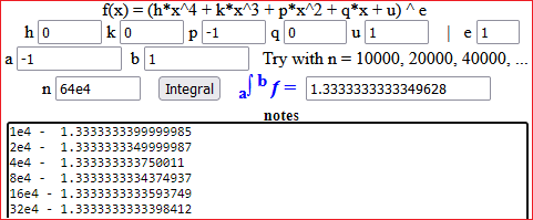
It is important to perform some approximate calculations of definite integrals with software to focus on the idea of integration, often obscured by the different concept of antidifferentiation.
At this point we can define the integral of any function F which is continuous on an interval [a,b],
or which is limited therein and continues on a finite set of intervals whose union is [a,b].
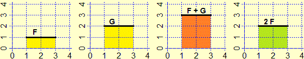
It is then possible to focus on other integration properties easily:
| ∫ [a, b] (F+G) = ∫ [a, b] F + ∫ [a, b] G | ∫ [a, b] (k F) = k ∫ [a, b] F |
The concept of defined integration must be introduced separately and before that of indefinite integration (or antidifferentiation),
themes which, then, will have to be connected by the fundamental theorem of calculus, on which we will dwell in a while. Let us dwell now on the concept of differentiation. | 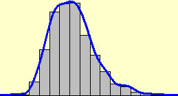 |
In the lower grade secondary school, and in the first two years of the upper school, students have already been introduced to the concept of slope
(or gradient) of straight lines (see).
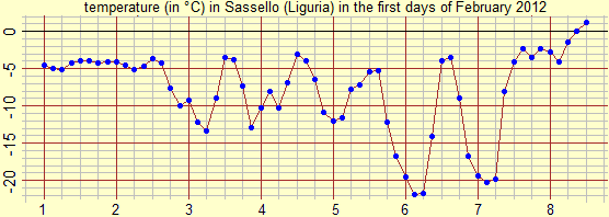
In the third class, the concept can be resumed starting from concrete situations.
For example, in the case of the following graph, students can be asked:
"in which period the temperature remained more or less constant?
around which integer value has it oscillated?
what was the average rate of change in temperature (measured in °C per hour) in the 6-hour interval in which it grew fastest?"
|
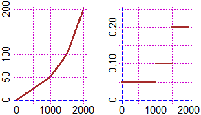
Then one can move from quantifying the slope to its graphical representation by referring to simpler graphs, such as the following. The first (which could represent, for example, how the level of the liquid introduced into the cistern shown on the side as the volume of it changes varies) is a sequence of straight sections linked together, flanked by the graph of its slope, which is a sequence of horizontal sections. The second is the graph of Then we can consider curves not made up of straight sections. | 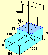 |
|  |
It is easy to focus on how to calculate the derivative of a function in x0 (i.e. how to define the slope of the line tangent in x0 to the graph of the function) using the concept of limit.
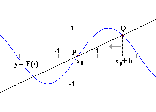
|  |
And it is very easy to obtain the derivatives of the functions x → xn: we refer to a trivial calculation in which it is sufficient to set h=0 to get the result.
| = |
| = |
| = |
| = |
|
It is appropriate, immediately (and returning to it later), to focus on a geometric characterization of this calculation:
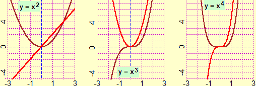
Again with graphic considerations, it is easy to develop that
In this way, in the third class, we are able to deal with the derivation of polynomial functions, essential for dealing
with the first formalizations of the laws of physics (see here for some reflection on this).
At the end of the third class, or in the fourth class, depending on the type of schools, the derivatives of other functions can then be introduced,
privileging the highlighting of the geometric meaning over formal justification.
However, before these developments, after seeing in simple cases how the definite integrals of some functions can be calculated directly, it is necessary to focus how the integration can be traced back to an antidifferentiation operation thanks to the fundamental theorem of calculus:
let f be continuous on [a,b]; if G' = f then ∫[a,b] f = G(b) − G(a)
There is no need to prove this theorem (which can then be addressed by those who continue their studies by choosing a scientific area), but it must be justified on some simple examples, such as the following, relating to
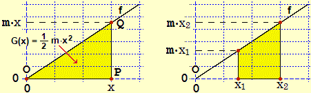
On the other hand, this example (assuming time as x, speed as f) corresponds to the calculation of the space traveled between time x1 and time x2 by an object that moves with speed that grows with constant acceleration.
The calculation of defined integrals using antidifferentiation is the most important aspect, which must be started in all schools, just as the term primitive (as a synonym for antiderivative - a primitive of F is a function that comes "before" the application of the derivation to F) and, possibly, the indefinite integral of F (to indicate the function
Even in subsequent developments relating to the functions of a variable (concavity, integration techniques, ...) it is necessary to distinguish the different levels to be reached in the various types of schools. In any case, it is necessary to privilege the understanding of ideas over training in techniques (end in itself, and temporary), which makes no sense in pre-university education. Rather, it is necessary to educate the reasoned use of the (reliable) resources available on the net. And it is necessary to overcome the fences between the different disciplinary areas (for example solutions of equations, inequalities and systems make use of concepts and tools presented in this paragraph; and concepts and tools related to these topics are used to study aspects discussed here). For some ideas about it see this worksheet.
We limit ourselves to remembering the strange use of ∫ f(x) dx to indicate a generic term
• in the case of the definite integral, the "integrated" variable is dummy (or mute):
one could write
• someone uses the indefinite integral to indicate a set of terms:
• the first convention is the most correct but it is less practical;
in general the second convention is used, occasionally making explicit, and sometimes not, the possibility of adding a constant,
that is, sometimes one writes
integral 6*x dx gives 3*x^2 + constant.
Always in scientific schools it is appropriate to focus, to prevent misunderstandings, the "calculative" differences between
differentiation and antidifferentiation:
while the derivatives of the "elementary" functions are still "elementary" the same does not happen for antiderivation;
for example the antiderivative of
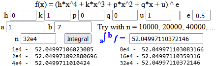
In all cases for the defined integration you can use the software (WolframAlpha or R for example), or this simple script, downloadable on your computer and editable to calculate any integral.
For example I can find that the integral between 1 and 7 of
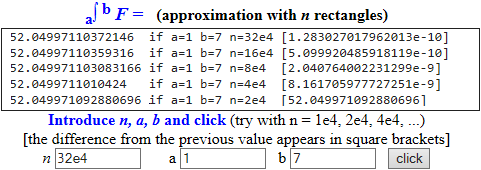 |
But for this integral the script seen above could also be used:
After focusing the idea that indefinite integration, as antiderivation, is an equation whose solution is a function (with a parameter),
in science-oriented schools we can mention the fact that, as such, it is also called differential equation",
and, possibly, mention other types of differential equations:
it is sufficient to rely on the software and the various free IT resources, always with a view to not dwelling on techniques at this level that are not comprehensible, and with the aim of giving the idea of possible developments to those who may wish to continue their studies in the scientific field.
For some ideas also in this regard see this this worksheet.
We repeat, it is not that certain topics should not be addressed because only later can they be studied in a more general and more in-depth way also from a technical point of view:
in significant cases, it is necessary to introduce these topics at a first level, then take them up again at a second level, and so on.
Even in the university education of those who continue their studies in the scientific field, only an intermediate level of formalization and application of them will be achieved.
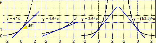
Funzioni esponenziale e logaritmo
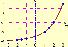 |
On the left, the graph of the function |
|
21.5 = 215/10 = 23/2 = (23)1/2 = √8 = 2.82842… 2−1.5 = 2−3/2 = 1/23/2 = 1/√8 = 0.353553… | |
|
With a calculating tool I obtain values also for other exponents;
for 2π with WolframAlpha I get for example: 8.82497782707628762385642960420800158170441081527148… Here is how the calculation could be done in these cases: |
| π = 3.1415926535897932384626433832795028841971693993751… | ||
| 23 = 8 | ≤ 2π ≤ | 24 = 16 |
| 23.1 = 10√(231) = 8.5741877002… | ≤ 2π ≤ | 23.2 = 10√(232) = 9.1895868399… |
| 23.14 = 50√(2157) = 8.8152409270… | ≤ 2π ≤ | 23.15 = 20√(263) = 8.8765557765… |
| ... | ... | ... |
| 23.141592 = 8.8249738290… | ≤ 2π ≤ | 23.141593 = 8.8249799460… |
| ... | ... | ... |
What we have seen now is the way the function x → 2x:
for rational x it is defined in the way illustrated at the beginning of this paragraph, in other cases it is defined as we have now seen, so as to be continuous, i.e. so that the outputs thicken with the thickening of the inputs.
The exponential function can be introduced in the first two years (as seen in the document relating to the first years of high school), but its meaning must be resumed in the third year, deepening it with the new concepts of mathematical analysis and intrerweaving it with the study of its function inverse, the logarithm function.
|
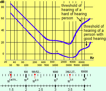
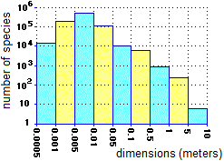
Among the practical applications of the concept of decimal logarithm, which students could find in other scientific disciplines and which are encountered in various contexts (including medical ones), there is its use as an extension of the concept of order of magnitude, which facilitates the description both of very large values (millions, billions, ...) and of very small values (millionths, billionths) and their graphic representation. The figure on the right illustrates its use for the representation of audiograms. Below it is shown how the animal species are distributed by dimensional classes (for example, we can see how there are few species of "large" animals and many of "small" animals). |
| ||
|
Seeing examples of use, such as these or others, is not a "luxury", but, rather, it is essential in pre-university teaching.
It is completely meaningless, and detrimental to the understanding of pupils and the construction of a reliable image of mathematics, to give definitions, to do repetitive exercises, … without first of all seeing examples of use (and role played in them) of various concepts and techniques introduced.
The idea that the pre-university school should build the "tools" and that the possibility of showing how to use them to model and solve problems should be left to the university is totally contrary, besides common sense, to the focusing of nature of science and culture and of the objectives of the school of "all".
Also in the reflections on this school bracket, let us report this "digression", fantastic but very concrete, on the concept of angle. Here various reflections are presented on the inopportunity of an axiomatic approach to the teaching of geometry. This was focused only at the end of the nineteenth century, especially with the aim of focusing on the different geometries that could be defined by changing some axioms. The so-called "Euclid's Elements" (not to be confused with "Euclidean geometry"), significant in the history of thought, certainly do not have the characteristics of what, in mathematics, is an axiomatic presentation: HERE is highlighted as well as the demonstrations of Euclid's first "theorems" are not acceptable.
We refer to the document relating to the first years of high school for discussion and exemplification of how to introduce and develop (with a view to a "spiral" shoot) the mathematization of space. There we have also exemplified how elements of three-dimensional geometry, elements of vector geometry and considerations on cartographic reproductions can be introduced, also by linking with the teaching of other disciplines. There we referred to this document (in Italian) for a more in-depth discussion of the setting of geometric teaching and for a rapid history of geometry itself (and for various exercises aimed at teachers).
Let us now recall, through some images and some comments, a few of the other issues that can be tackled in the last years of high school. The goal of a large part of the new contents to be developed in this school segment is not so much that a good technical mastery of them is acquired, but that of giving to understand, also operationally, their role in the social and productive context. The main purpose of the school, especially in recent decades, is cultural, not professional. Also in relation to the rapid transformations that go through the world of work and the economy, more orientation skills, understanding of processes, adaptation to technological changes than hyperspecialized information are required for insertion into the world of work. We need to ensure that the links between techniques and general concepts are understood, not to teach abstract knowledge and to train repetitive practices separately. This is the challenge that the school must face, if it does not want to continue in its progressive cultural and social decline.
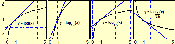
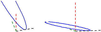
Let's start from the concept of distance. In common language the distance is between objects and figures, not between points. What sense does it make in school to confine yourself to the distance between points?
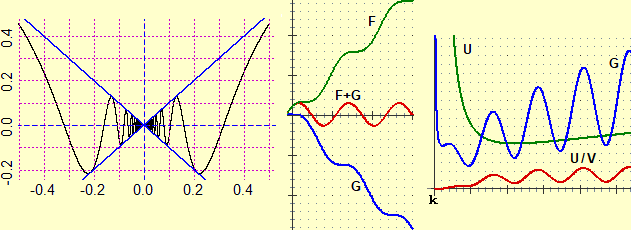
The image (1) illustrates the distance between two curves (or between two islands): it is the minimum between the distances of two generic points that lie on them.
In the image (2) the distance between the curves A (a curve having y=1 as an asymptote) and B (the straight line y=1/2) is 1/2, but it is not the minimum of the distances between two points on A and on B:
they form an interval
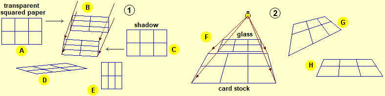
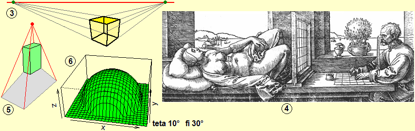
It is necessary to consolidate some three-dimensional geometry concepts, both those mentioned in the document relating to the first years of high school, and others related to the concept of perspective (which should have already been focused on in basic school and on which synergies could be realized with the teaching of other disciplines: drawing, art history, …); they are very important both in the history of mathematics and in its applications, increasingly present in everyday life. It is not a question, also in this case, of making in-depth (and internal mathematical) treatments, but of pointing out (resorting to the indispensable use of the computer) ideas and concepts, as highlighted by the following figures. The levels of deepening can then be very diversified in relation to the type of school and the willingness to collaborate by teachers of other subjects.
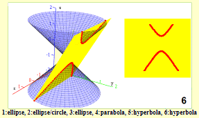
Conics do not constitute a "fundamental" mathematical theme from a "technical" point of view with respect to the basic knowledge to be developed. However, it is culturally important to have an idea of the connections between various areas of mathematics that conics highlight. Some of the images present here recall the contexts in which parables, ellipses and hyperbolas, thought of as independent curves, have found many applications since antiquity; these are subjects that can be easily tackled by studying curves in general, also linking to other disciplines, in some aspects since the lower secondary school. The second, third and fourth of the following figures illustrate, instead, how the term "conics" can be introduced, towards the end of high school, in all schools: we can represent conics as an intersection between a cone and differently arranged planes, we can highlight that if we look at a conic from the vertex of the cone it appears to be circular anyway, we can highlight that with just one glance we cannot distinguish which type of conic we are observing.
 |  |  |
 |
|
 |
In scientific schools it is possible to study how to represent all the conics analytically and, in case, how to represent them also in polar form (see the final part of the document to which you have been addressed a little above; for further details see here).
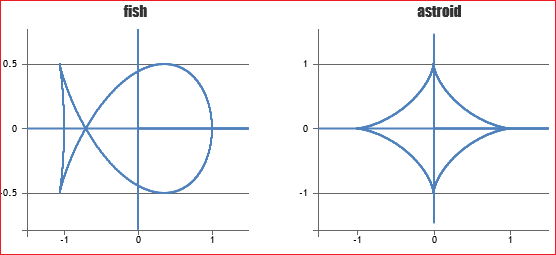
But it is perhaps more important to give an idea of the many other curves that can be described with simple mathematical formulas (see).
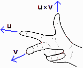
On the topics of three-dimensional geometry that can be addressed in the final part of high school, we have already focused just above (discussing perspective and conics) and in the document relating to the beginning of high school (see). Further developments to be addressed in all schools, with elementary motivations, are the volumes of some simple figures (parallelepipeds, cylinders, pyramids, cones, spheres) and, in particular in those with a scientific orientation, three-dimensional vectors.. To get an idea of the insights that can be treated in scientific schools, see for example here. An animation that concretely exemplifies how the theme of non-Euclidean geometry could be addressed, and gives some bibliographical indications: Walking on the spheres.
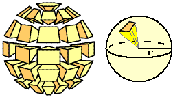 |  |
Statistics and theory of probability
As mentioned in the previous sections, the fact that statistical and probabilistic tools are to be used (and whose outcomes are to be interpreted) in contexts that are not purely mathematical is perhaps the reason why they are often overlooked (or developed in occasional and not at all correct ways) by teachers;
all this despite that, in the first school levels, this area of mathematics involves only tools common to other sectors of the discipline.
Up to the previous section (see) we discussed statistics and probability in separate paragraphs, while in this one, referring to the final years of high school, we deal with them in a more intertwined way and we explain the link between them through the "central limit theorem", of which the pupils, in previous years, implicitly perceived the existence
(they understood that in a statistical experiment with increasing tests the ratio between the number of favorable exits and total exits tends to stabilize on the probability).
Recall that here there are links to programs that can be used for statistical processing, and that here you can find a brief history of probability theory.
If this has not already been done in the two-year period, it is necessary to focus the fact that a discrete random variable can be "not finite".
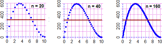
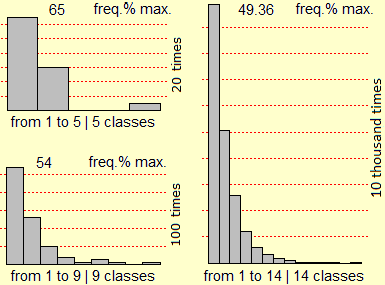
The following figure shows the histograms relating to several results of the experiment (handmade and simulated with the computer) of counting how many times it is necessary to flip a balanced coin to get the "head" outcome.
As the number of tests increases, the frequency distribution histogram tends to become an unlimited figure, but in any case with a finite area, equal to 1
(it should be pointed out to pupils that this is not a strange thing: since basic school they know that 1/9 = 0.111… = 1/10 + 1/100 +
 |  |
|
1/2 + 1/2² + 1/2³ + … = 1 |
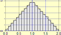 |
We can move from the case of throwing two dice to the study of the sum of two numbers between 0 and 1 obtained with the "random number generator". We pass, naturally, from a histogram to a triangle, from a sum to an integral (see the figure on the left). The transition from histograms to continuous density functions, on the other hand, can be a context for the introduction of integration which may precede the one discussed above. Another example: the histogram of distribution of arrival times in a television sale between one phone call and another and, superimposed, the graph of a function that seems to approximate it. Phenomena of this type (such as the temporal distance between coming to the traffic light of a car and that of the next, in the case of a traffic light preceded by a long stretch of road without impediments) have an exponential distribution. | 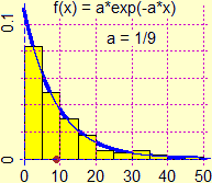 |
|
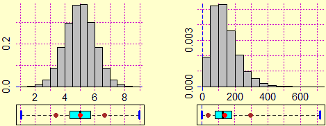
Above some examples of distribution laws. The last histogram represents a Gaussian distribution law which, beyond what is often made to believe by pupils, does not occur very often in nature (for example the following phenomena are distributed roughly in this way:
the heights of adults of a given sex belonging to a certain racial group,
the lengths of fish of a particular species, …,
recordings by several people with a manual stopwatch of the same time duration, …).
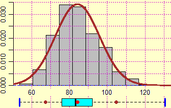
On the right, for example, the distribution histogram of the weights recorded in Italy at the first contingent of the call-up visits (of males in their twenties) in 1987 is reproduced, which, as is evident, has no Gaussian trend. Why is Gaussian distribution important? Because the average of almost all random phenomena, however distributed, does have a Gaussian trend, and this allows us to estimate the precision of the obtained average value or, if a phenomenon is being simulated, the precision of the obtained estimate of the probability that it happen. | 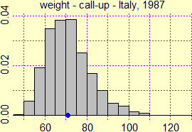 |
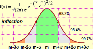 |
More precisely, knowing that knowing that the detected weights are N = 4170 and that their average is m = 70.977, we have that, if I repeated the test many times with N other individuals of the same category taken at random, I would obtain other values of the average which in each case would be distributed according to a Gaussian, such as the one shown alongside;
there σ = sd/√N, where sd is the so-called "experimental standard deviation" (square root of the division by N-1 of the sum of the squares of the deviations from the mean value), that is σ = 0.163 (see here for details, of to which at least the teacher must be aware).
I can conclude that in 1987 the average weight (in kg) of an Italian male in his twenties is 70.977±0.163, with a probability of 68.3%, and that it is 70.977±0.163·3 = 70.977±0.489 (71±0.5 kg) with a probability of 99.7% (i.e. with practical certainty). Another example: if with a high sensitivity measuring device I get the 7 values (in a given unit of measurement) 7.3, 7.1, 7.2, 6.9, 7.2, 7.3, 7.4, I can calculate the average (7.2000…), the standard deviation (0.061721) and its triple (0.185), and conclude that with 99.7% probability the "true value" of the measure is 7.200±0.185. |
The property now referred to constitutes the central limit theorem, which intertwines probability and statistics and is the basis of all the applications of this area of mathematics (also of the realization of the surveys that the television media propose to us, often badly).
Incidentally, we observe that the fact that the average of N random variables, with the same distribution law of average m, tends (in probability, in the manner described above) to m as N increases, is called law of large numbers".
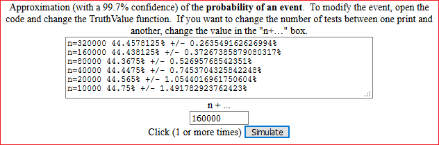
This property is also used to evaluate the results of a simulation (here are some examples).
It is not important that students, especially from schools that are not scientific or technological oriented, memorize procedures and techniques. It is important that they understand the main ideas, that they realize that not everything is Gaussian, and that they rely on software (R - see here - or, for simple things, WolframAlpha) to deal with some significant situation. Rather, it is good to give simple examples that constitute "vaccines" with respect to the misconceptions spread by the mass media (and sometimes also by the world of education). For example we can take data distributed in a Gaussian way and consider the cubes of the same data, observe how the shape of the distribution histogram changes, note that while the median of the new data is the median of the first data, this does not happen for the average; and then, make transfers to contexts (if in a population of fish or in a collection of beans the lengths are distributed in a Gaussian way, this cannot happen for their volumes and, therefore, not even for their masses).
| ||||||
Here you can find a simple script to integrate the Gauss distribution:
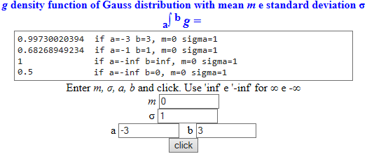 |
In-depth insights that can be addressed in scientific or technological schools are discussed in the next paragraph.
Both in the discrete and in the continuous case, to calculate the probability of events you can use this simple script, downloadable on your computer and editable. For example, I can evaluate the probability that by rolling three balanced dice you will get at least 2 equal exits (and conjecture that it is 4/9, and then look for a demonstration):
Relationships between two random variables
The main applications of statistics, in every field (medical, economic, biological, physical, ...), are aimed at studying the links between different quantities that vary randomly.
Also in this case it is necessary to give all pupils an idea of this area of employment, not only to give them tools for any future choices in the continuation of their studies, but, above all, to offer them cultural elements to interpret everyday phenomena, and critically evaluate the information and interpretations provided by the "media".
No advanced knowledge is needed to acquire this awareness. As we have said several times, it is not important to memorize procedures and techniques at this school level.
In many types of schools it is possible to limit oneself to two examples of situations, which do not involve advanced knowledge (but it is necessary to focus that in other cases it is necessary to resort to more sophisticated tools).
First example. Discussing the model concept (in the previous document) we saw that the link between the DS distance along the road and the DA distance in a crow flies from Genoa to other places in Northern Italy can be addressed by collecting data relating to the minimum road distances from Genoa of the other provincial capitals (of Piedmont, Lombardy and Veneto) and those relating to the distances in the crow flies, graphically representing them and trying to approximate the points with a straight line. This approach is illustrated on the side.
I get a straight line that passes around the point | 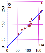 |
# For example, using R (see here):
da = c(55, 70,155,160,155,115,105,165,110,115, 85,165,110,155,105)
ds = c(85,115,205,230,185,185,145,240,140,155,125,290,170,195,135)
Plane(0,170, 0,300); POINT(da,ds, "brown")
regression(da,ds,0,0)
# 1.42 * x
f = function(x) 1.42*x; graph1(f, 0,200, "blue")
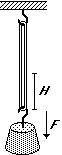
Second example. I hang different objects from a rubber band.
Let F be their weight (in g) and H (in mm) the elongation of the elastic.
I can determine the values of H with the precision of 2 (mm) and those of F with the precision of 5 (g).
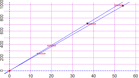
I can represent the experimental points with rectangles.
I know that (in the weight range considered) between H and F there is a linear relationship
|
| ||||
| (990-5)/(52+2) = 18.24074 (710+5)/(39-2) = 19.32432 F = k·H, k = 18.8±0.6 | |||||
The following images recall other topics that can be tackled (using free standard software, such as R) in scientific schools, favoring an understanding of the conceptual aspects compared to the technique.
| In a case like the previous one, but in which I do not know the precision of the various measures, I can determine the interval in which the slope of the straight line falls with 90% probability (or with another probability). In this case I get that it is between 18.03658 and 19.35311. |
|
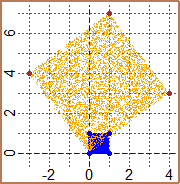
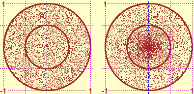  |
What does "take at random" mean? Even in the two-dimensional case it depends on the distribution law according to which it is done. On the left, the representation of two different ways to generate the fall of a point in a circle of center (0,0) and radius 1. |
| Let's consider the images on the side. On the left, there is the graphical representation of the distribution of (X,Y) with X and Y heights of a randomly drawn man and woman. In the center, the one with X and Y husband and wife heights of a randomly drawn couple, and, on the right, a possible experimental dispersion graph of the same distribution (taller men tend to marry taller women: it is not true that love is blind!). In both cases X and Y are dependent on each other, in the second case they are also correlated to each other. | 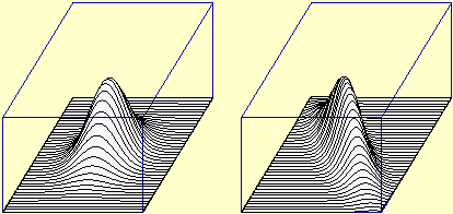  |
The correlation coefficient between two sets of paired values expresses a value that is as close to 1 or to −1 as the two sets of values can be approximated with a linear relationship of the type
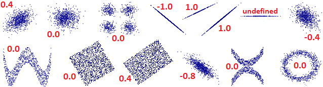 |
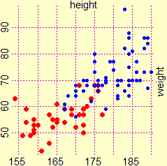 |
The points in the diagram alongside represent heights and weights of the students of a university course; they are very aligned (there is a high correlation coefficient, 0.78).
But if we observe only the (red) points corresponding to the female population we have a different impression (the correlation coefficient is 0.52). The statistics only highlights the numerical relationships between the data, not the cause-effect relationships, for which specific knowledge and studies of the area involved are needed! |
An investigation of the weight of males between 45 and 55 years of a certain state gives the results graphically represented below on the left. The detections are 825.
An attempt was made to superimpose a Gaussian with the same mean and standard deviation on the histogram.
There seems to be a reasonable correspondence. Can I assume that the trend is Gaussian?
Absolutely not!
In fact, to evaluate this correspondence, a certain value is calculated, called χ2, which depends on the data and their number (we obtain 27.07). Then we compare it with the graph (easily traceable with the computer) which represents how χ2 would be distributed if the trend were actually of this type (ie Gaussian).
Its median value is seen to be 7.34, much less than 27.07, as is the 95th percentile (15.51).
The hypothesis that the trend is Gaussian is certainly to be discarded: 27.07 is a highly improbable value.
 | 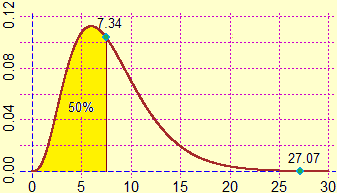 2.73−5% 5.07−25% 7.34−50% 10.22−75% 15.51−95% |
Thorough examination of all these aspects can be found here.
Insights on mathematical analysis
|
There are other aspects of mathematical analysis that can be presented in all types of school and that can be further explored in science-oriented ones.
The first is the possibility that a function that is several times derivable can be approximated around a point by a polynomial function.
The most useful cases are illustrated alongside (for | 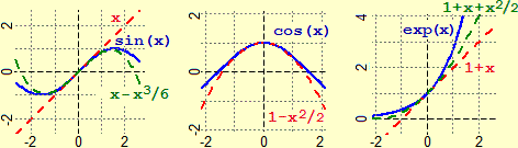 |
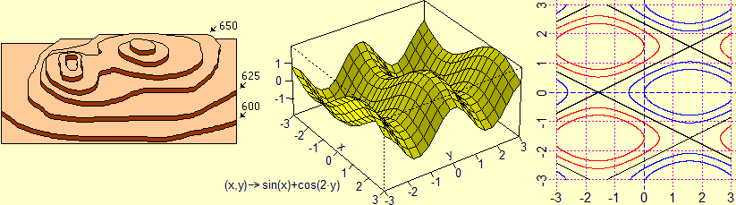
In the first years of school pupils became familiar with many multi-input functions (sum, product, average, ...), and studied many others in the following years. At the end of the high school it is good that everyone sees, with simple examples, how the real 2 input and 1 output functions can be graphically represented (generalizing cases of analogous 1 input functions):
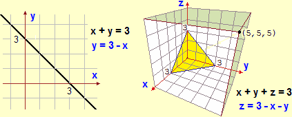
It is possible to focus the connections with the reading of the contour lines of a map and, if desired using the computer, view the graphs of some functions and the relative contour lines. In scientific or technological schools it is possible to explore the connections with the theme of space and with that of the relationships between random variables, discussed in previous paragraphs. For some ideas on the developments that can be tackled in these schools (Hessian, gradient, Fourier series, ...) see for example here and here.
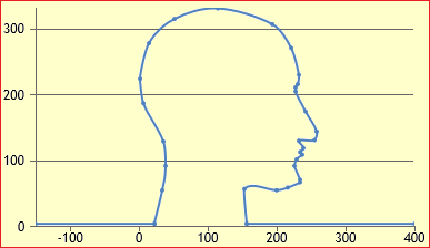 |
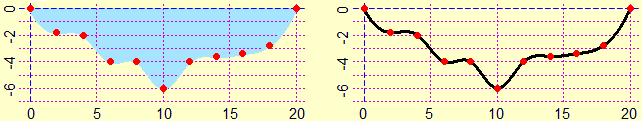
There are also significant applications that can be mentioned and whose "at the back mathematics" can be easily understood, such as cubic splines:
curves consisting of sections of third degree polynomial curves that join so that the first and second derivatives from the right and from the left are equal
(see). On the left, a figure (see here). Another example: the section of an artificial basin starting from some depth measurements: |
More
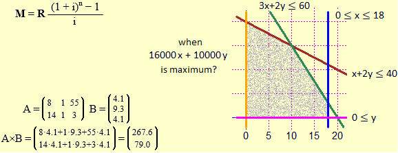
We mention other topics that can be addressed in last years by some schools with an economic or technical orientation, where the use of the software is decisive:
financial mathematics and linear programming (see here and here), and matrix calculus, with its varied uses in many areas of mathematics (see here and here).
Educational differentiations, and final considerations
In discussing the first two years, we observed how the level of deepening can be different as the type of school varies, and how the intertwining with the other disciplines can also differ. In the final years, as we have seen, there are different levels of depth that can be reached; and also the themes that can be dealt with differ according to the school curriculum. In all types of schools, however, it is necessary to give an idea of the various uses of mathematics, so that any choices for continuing the studies are not oriented by a small and distorted vision of the discipline, a vision that pushes either to the choice of university studies of mathematical area by people who think of it as something detached from other forms of knowledge, based on mechanical activities and on the repetition of stereotyped forms of reasoning, or to the choice of other studies by curious people, interested in the intertwining of different areas, in the search for problem solving strategies and in the understandable communication of the procedures developed.
We have repeatedly observed how the software, chosen in an appropriate way, can facilitate the didactic management of many contents: it allows to face, especially in the last years of high school, topics conceptually, but not technically, within the reach of the pupils, and with different levels of deepening in different school situations. It is important to focus how the circulation of multimedia aids is one of the aspects that most challenge the current role of the teacher: it is inevitable that the teacher is technologically "less advanced" than the pupils, but this must not be resolved on his part (as often happens) in avoiding new technologies or in relying on obsolete aids that he learned to use several years before. It is necessary to relate differently with the pupils, it is necessary to get "explained" by them what are the new technologies they use and, in return, to give them the knowledge and the tools to master these technologies culturally. In particular, the teacher must "teach" what, how, where, ... to search through internet and how to evaluate the things found there.
Mathematics has the specificity of not being characterized by a particular area of problems or phenomena that it tries to model (such as physics, history, linguistics, …), but by the typology of artifacts that it uses for the construction of models, and which are used in all other disciplines. We have seen that concepts born as "abstractions" starting from concrete situations gradually become "concrete" objects from which to start to develop new abstractions, in an endless spiral. Mathematical knowledge, which arises from modeled contexts, is organized, unlike other disciplines, not on the basis of contexts, but of the relationships and structural analogies between its artifacts. The (operational) acquisition of the role and meaning of this abstract nature must be gradual and, simultaneously, the function of definitions and demonstrations must be gradually focused. It seems obvious (but it is not for the authors of the most popular textbooks) that the goal of the school must be the construction of the meaning of these, not the temporary and misunderstood jumble of sentences, formulations and recipes.
Obviously, it would be necessary that, subsequently, at university level, one did not proceed, as unfortunately it often happens, with arrogance and presumptuousness, without any reflection on the objectives of previous school levels, without reflecting on the nature (technical and historical, in short "cultural") of definitions, demonstrations, relationships between the various subject areas, with attitudes towards students who, perhaps a bit caricaturally, we could represent with phrases like "let's start from scratch, throw everything you have studied overboard: now let's see what mathematics is! ".
And this, unfortunately, applies, not infrequently, also to courses oriented to the teaching of mathematics, which often focus only on basic knowledge, often presented separately from each other, and which almost always neglect the reflections on the concepts dealt with in high schools, which instead could trigger considerations on the different ways in which the concepts must be presented in the different brackets of education, considerations which, moreover, can refer to still "hot" educational experiences for students.
Finally, as noted several times, it must be taken into account that the continuous renewal of mathematics, its uses, its interactions with other disciplines, the available technologies, the opportunities offered by the network require that part of the contents and techniques, which have become obsolete, are gradually scaled down or thrown overboard to give space to new content and new mathematical techniques, and to attitudes that allow you to find, select and use what the new media offer. Mathematics is alive.