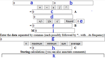
pocket calculator-1
functions
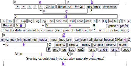
pocket calculator-2 help
pocket calculator-1 | Math functions | pocket calculator-2 help |
a a' a" a''' d d' d" e f g g' g" g''' g'''' g''''' i j j' k k'
Note. You can get results like this: 0.5-0.4 = 0.09999999999999998 as the calculations are done using base 2 instead of base ten (and 0.4 in base 2 has not a terminating representation: 0.011001100110011001100110011…; therefore 0.4 is not represented exactly in the calculation). But,in this case, with "Round [16]" you get 0.1. See sixteenth example. Spreadsheets proceed in the same way but in a "hidden" way, often producing results that are not easily controllable: see fourth example.
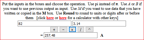
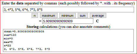
1-First example (with pocket calculator-1):
A wheel has a diameter of 82 cm. What is its circumference?
A typical example of an incorrect answer: the use of 3.14 and thinking that 82 cm is an "exact" measurement.
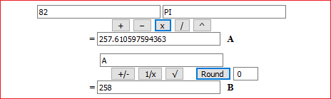
Or correctly rounding the answer with 3 digits (Round "0" rounds to units), but using 3.14:

The correct answer:
2-Second example:
A school class in a winter month detects the outside temperature on each school day at 9 o'clock:
I round to tenths:

3-Third example:
Unlike the behavior of pocket calculators, the computer operates with numbers in a somewhat different way, so the results of the operations may differ by a few units on the last (the 17th) digit. However, they are more digits than are usually needed. With this calculator we can round numbers.
Some example.
1 / 3 = 0.3333333333333333
10 / 3 = 3.3333333333333335
3.3333333333333335 round to 14^ digit after units: 3.33333333333333
√3(-8)
-8 ^ 0.3333333333333333 = -1.9999999999999997
-1.9999999999999997 round to 15^ digit after units: -2
Let's compare the values of these two numerical terms: (19/6177)^2 and (10119/355 - 12398/435)^2.
19 / 6177 = 0.0030759268253197345
0.0030759268253197345 ^ 2 = 0.000009461325834721535
10119 / 355 = 28.504225352112676
12398 / 435 = 28.501149425287355
28.504225352112676 - 28.501149425287355 = 0.003075926825321318
0.003075926825321318 ^ 2 = 0.000009461325834731285
Only 11 digits are equal while the two terms are equivalent. Similar problems also happen with the usual calculators.
Let's see how we could check the equivalence of the two terms:
355 * 435 = 154425
10119 * 435 = 4401765
12398 * 355 = 4401290
4401765 - 4401290 = 475
10119/355 - 12398/435 = 475/154425. With this script I can find that:
475/154425 -> 19/6177
With this script I can find that the period of 19/6177 is 140 digits long:
0.003075926825319734498947709243969564513517888942852517403270195887971
50720414440666990448437752954508661162376558199773352760239598510603853
00307592682531...
If I want (and if I have a lot of time available) I can find the period of (19/6177)^2 = 361 / 38155329 (it is long 288250 digits):
0.000009461325834721540469484616421470248625034788718503777021553136129425066679
41455831765990014134067616085815955092406620317701886412773429368149335050943997
88821110676309461255071342721222506035788605046492981360480471810372805329499321
05158888814718384422789278006225552399246773628920877605327423595272890976775485
28018196357316169387505477937302021429300216491384466898450803556169047841259604
91652424226246352115061044290825011625505836943510564408971548902120592381735196
15045122530590681055325194548840084696950195344928096413478704377047829937464305
44472568956226271826931435973203114039456978604482744730100479542451330979219180
...
4-Fourth example:
843.27−843.23 and 5555.1251−5555:
see here.
5-Fifth example:
Human body weight (peso corporeo); 4170 Italian males in their twenties, in the year 1990. (here).
We have seen how to obtain the following histogram and the following elaborations:
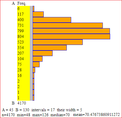
We can get (with this version - "pocket calculator-2"):
I put the data in (g):
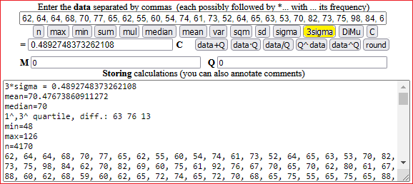
Values are rounded to units. The central 50% of the data is in [63, 76], an interval of amplitude 13. The average weight (of Italian males in their twenties, in the year 1990) is 70.48±0.49 kg, or 70.5±0.5 kg.
6-Sixth example:
From 2007 to 2012, employment had the following percentage changes (each calculated with respect to the previous year): 1.6, 2.8, 1.3, -0.8, 0.9, 1.7. What was the overall percentage change?
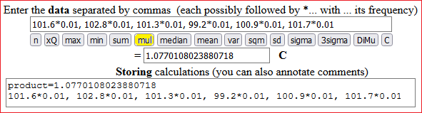
I get 1.077011, or 107.7%: there was a positive change of about 7.7%. I put "about" as the data are rounded and there may be changes in the last digit due to rounding.
7-Seventh example:
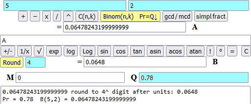
8-Eighth example:
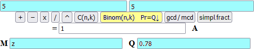
In a large number of experiments it is obtained that a certain poison kills 78% of the mice on which it is tested. If used on a group of 5 mice, what is the probability that 0, 1, 2, 3, 4, 5 mice are killed?
The probability of a mouse dying is 0.78. So we have to consider the binomial law
To calculate
Pr = 0.78 B(5,5) = 0.28871743680000006 round to 4^ digit after units: 0.2887, 28.87%
Pr = 0.78 B(5,4) = 0.40716561600000006 round to 4^ digit after units: 0.4072, 40.72%
Pr = 0.78 B(5,3) = 0.22968316799999997 round to 4^ digit after units: 0.2297, 22.97%
Pr = 0.78 B(5,2) = 0.06478243199999999 round to 4^ digit after units: 0.0648, 6.48%
Pr = 0.78 B(5,1) = 0.009135983999999998 round to 4^ digit after units: 0.0091, 0.91%
Pr = 0.78 B(5,0) = 0.0005153631999999998 round to 4^ digit after units: 0.0005, 0.05%
If in [M] I put "z" (zero) the sum B(n,0)+B(n,1)+...+B(n,k) is calculated. Example 1:
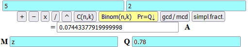
Example 2:
9-Ninth example:
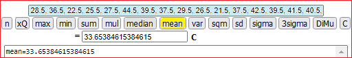
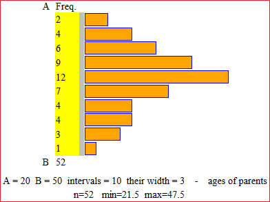
Pupils in a 4th grade class collect the ages of their parents when they were born. Below are the data. What was the average age of the parents when the pupils were born?
28, 36, 22, 25, 27, 44, 39, 37, 29, 26, 21, 37, 42, 39, 41, 40, 45, 24, 34, 28, 41, 32, 32, 30, 45, 24, 33, 31, 29, 34, 26, 33, 34, 28, 41, 30, 35, 37, 29, 39, 24, 33, 31, 36, 32, 32, 35, 29, 33, 47, 34, 31
We can get (with this version):
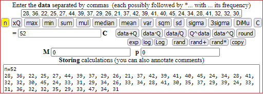
The data is truncated. To process them correctly we need to add half a year to all ages (a 32-year-old person has an average age between 32 and 33).
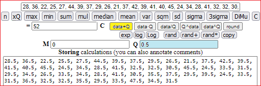
With [copy] I introduce the transformed data:
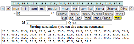
The mean is 33.7:

We have seen how to obtain (with the transformed data) the following histogram:
10-Tenth example. Rounding should only be done at the end:
In many manuals, especially in the biological field, but also in the physical field, still (in the XXI) many complex calculations are performed by rounding off the intermediate results, gradually losing information; but in the end these manuals round off the result with many figures more than the legal ones (once, up to the middle of the twentieth century, in the absence of convenient means of calculation, this was often the case, but generally the rounding was done correctly ...). An example from a famous manual of mathematics for the life sciences.
To evaluate the density of trees in a park, the number of trees per hectare that are present in 5 differently placed sample areas are counted, obtaining:
Size in hectares of the area 1.50, 2.30, 1.75, 3.10, 2.65
Number of trees present in it 20, 31, 43, 58, 29
Determines the mean and standard deviation of the density (number / hectare).
Developing the calculations the manual finds as answers 16.2 and, therefore, 5.491.
Let's do the calculations with the calculator:
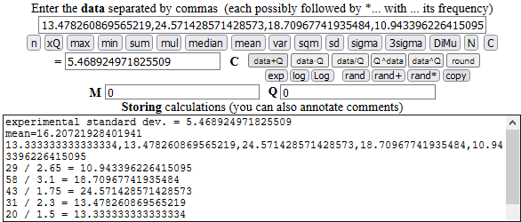
The extended experimental standard deviation value is 5.468924971825509, the rounded value is 5.469, very different from that indicated in the manual (manual that to do the calculations misused - and makes the students use - an expensive numerical calculation software!).
11-Eleventh example. Round up a sequence of number:
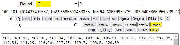
We transform a sequence of numbers (e.g. men's high jump records every 4 years from 1932 to 1996: 203, 207, 209, 211, 211, 211, 215, 222, 228, 228, 229, 232, 236, 239 , 243, 244, 245) into index numbers (let's set the first data equal to 100 and transform the others proportionally) and then round the index numbers to the second digit after ".".
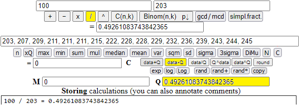
I put the data sequence (separated by ",") in the "data" box. I calculated 100/203. I copied the result in box Q. So I clicked [data·Q]..
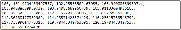
With [copy] I paste the index numbers obtained and, finally, I put 2 next to [Round] and click [round]:
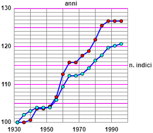
If I similarly transform the data on female records (165, 165, 166, 171, 171, 172, 176, 186, 191, 191, 194, 196, 201, 207, 209, 209, 209) and graph everything ( using this script) I get:
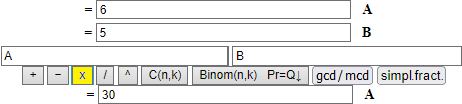
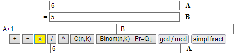
12-Twelfth example. Enter expressions instead of numbers.
I can introduce in the cells instead of single numbers terms that contain more numbers (the only operations allowed are +, *, -, / and those of the type "Math").


| 36 + 1 |
| ————— |
| 53 · 24 · 0.3 |


                  Usable "Math" Functions:
abs(a)     / |a|                            log10(a) / log of a base 10
acos(a)    / arc cosine of a                max(a,b)
asin(a)    / arc sine of a                  min(a,b)
atan(a)    / arc tangent of a               pow(a,b) / a to the power b
atan2(a,b) / arc tangent of a/b             random() / random n. in [0,1)
cbrt(a)    / cube root of a                 round(a) / integer closest to a
ceil(a)    / integer closest to a not < a   sign(a)  / sign of a
cos(a)     / cosine of a                    sin(a)   / sine of a
exp(a)     / exponential of a               sqrt(a)  / square root of a
floor(a)   / integer closest to a not > a   tan(a)   / tangent of a
log(a)     / log of a base e                trunc(a) / integer portion of a
log2(a)    / log of a base 2                PI       / π

cosh(a),sinh(a),tanh(a), acosh(a),asinh(a),atanh(a)    hyperbolic functions

      Note:   M%%N is the remainder of M/N,   != is "not equal"
|
Other examples:

cbrt(27000)           output: 30
max(39/7, 6, 79/14)   output: 6
random()              output: 0.9055236689456472
random()              output: 0.8572220665948553
random()              output: 0.16923464144969635
        The roll of two fair dice:
trunc(random()*6+random()*6)+2  output: 4
trunc(random()*6+random()*6)+2  output: 8
trunc(random()*6+random()*6)+2  output: 6
trunc(random()*6+random()*6)+2  output: 9
trunc(random()*6+random()*6)+2  output: 11
13-Thirteenth example. Negative-based powers
5 [^] -2 -> 0.04
-5 [^] -2 -> 0.04
-5 [^] -3 -> -0.008
5 [^] -3 -> 0.008
125 [^] 1/3 -> 5
125 [^] -1/3 -> 0.2

-2 [^] -1/3 -> NaN                                                                1 dispari
-2 ^ (-1/3) = -2 ^ -1 ^ (1/3) = (-1/2) ^ (1/3)
1/2 [^] 1/3 -> 0.7937005259840998
[+/-] 0.7937005259840998 -> -0.7937005259840998

-2 [^] -4/3 -> NaN                                                                4 pari
-2 ^ (-4/3) = -2 ^ -1 ^ (4/3) = (-1/2) ^ (4/3) = (1/2) ^ (4/3)
1/2 [^] 4/3 -> 0.3968502629920499

(-5/3)^(-5/3) = (-5/3)^(-1)^(5/3) = (-3/5)^(5/3) = -(3/5)^(5/3) = -0.426827...    5 dispari
(-2/3)^(-2/3) = (-2/3)^(-1)^(2/3) = (-3/2)^(2/3) = (3/2)^(2/3) = 1.31037...       2 pari

(-2)^(-1/4), (-5/2)^(-5/2), (-a)^(m/n) [-a < 0, m/n simplified, n even] are not defined

WolframAlpha
(-2)^(-1/3)  (choose "Use the real valued root")
= -2^(2/3)/2 = -0.7937005...

(-5/2)^(-5/2) (I cannot choose "Use the real valued root")
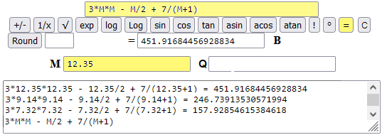
14-Fourteenth example. Use of M and other "letters"
The value put in (i) can be used in the "input" windows (both the 2 input - (a),(b) - and the 1 input one - (d)) using the letter M (it is automatically transformed into the value it represents). In (d) M can also be used within a more complex term (see); an example: 3*M*M - M/2 + 7/(M+1)
Another example: study of lim x → 0 cos(sin(1/x)*x). I put cos(sin(1/M)*M) in the "1 input" window and 1, 1e-1, 1e-2, ... in the "M" window:
cos(sin(1/1e-8)*1e-8) = 1 (0 after units) [read from bottom to top]
cos(sin(1/1e-7)*1e-7) = 0.9999999999999991 (0 after units)
cos(sin(1/1e-6)*1e-6) = 0.9999999999999387 (0 after units)
cos(sin(1/1e-5)*1e-5) = 0.999999999999936 (0 after units)
cos(sin(1/1e-4)*1e-4) = 0.9999999995329992 (0 after units)
cos(sin(1/1e-3)*1e-3) = 0.9999996581351323 (0 after units)
cos(sin(1/1e-2)*1e-2) = 0.9999871797192685 (0 after units)
cos(sin(1/1e-1)*1e-1) = 0.9985205700839945 (0 after units)
cos(sin(1/1)*1) = 0.6663667453928805 (0 after units)
cos(sin(1/M)*M)
Another example: the derivative of x³+1 in 4 (M = 1, 1e-1, 1e-2, ...):
( (pow(4+1e-5,3)+1)-(pow(4,3)+1) )/ 1e-5 = 48.00011999748221
( (pow(4+1e-4,3)+1)-(pow(4,3)+1) )/ 1e-4 = 48.00120000993502
( (pow(4+1e-3,3)+1)-(pow(4,3)+1) )/ 1e-3 = 48.01200100001779
( (pow(4+1e-1,3)+1)-(pow(4,3)+1) )/ 1e-1 = 49.20999999999992
( (pow(4+1,3)+1)-(pow(4,3)+1) )/ 1 = 61
( (pow(4+M,3)+1)-(pow(4,3)+1) )/ M
That is with ( (pow(4+M,3)+1)-(pow(4-M,3)+1) )/ (M*2)
( (pow(4+1e-4,3)+1)-(pow(4-1e-4,3)+1) )/ (1e-4*2) = 48.00000000997784
( (pow(4+1e-3,3)+1)-(pow(4-1e-3,3)+1) )/ (1e-3*2) = 48.000001000005454
( (pow(4+1e-2,3)+1)-(pow(4-1e-2,3)+1) )/ (1e-2*2) = 48.000099999998724
( (pow(4+1e-1,3)+1)-(pow(4-1e-1,3)+1) )/ (1e-1*2) = 48.009999999999984
( (pow(4+1,3)+1)-(pow(4-1,3)+1) )/ (1*2) = 49
( (pow(4+M,3)+1)-(pow(4-M,3)+1) )/ (M*2)
Another example: the recursively defined sequence P(0) = 1, P(n+1) = P(n)*1.5.
We can use
(d) and (f).
Put 1 in (f), B*1.5 in (d).

If you click [=] you will gradually get in B:
1 1.5 2.25 3.375 5.0625 7.59375 11.390625 ...
7.59375 * 1.5 = 11.390625
5.0625 * 1.5 = 7.59375
3.375 * 1.5 = 5.0625
2.25 * 1.5 = 3.375
1.5 * 1.5 = 2.25
1 * 1.5 = 1.5
B * 1.5
Another: y(0) = 1, y(n+1) = (y(n) + T/y(n)) / 2 y(n) → √T T = 9:

(3.000000001396984 + 9/3.000000001396984) / 2 = 3
(3.00009155413138 + 9/3.00009155413138) / 2 = 3.000000001396984
(3.023529411764706 + 9/3.023529411764706) / 2 = 3.00009155413138
(3.4 + 9/3.4) / 2 = 3.023529411764706
(5 + 9/5) / 2 = 3.4
(1 + 9/1) / 2 = 5
(B + 9/B) / 2
Another: the series 1 + 1/2 + 1/3! + 1/4! + ...
I use B gradually adding "/2", "/3", "/4", ...
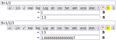
1.7182818284590453+1/2/3/4/5/6/7/8/9/10/11/12/13/14/15/16/17/18 = 1.7182818284590455
B+1/2/3/4/5/6/7/8/9/10/11/12/13/14/15/16/17/18/19
1.7182818284590453+1/2/3/4/5/6/7/8/9/10/11/12/13/14/15/16/17/18 = 1.7182818284590455
B+1/2/3/4/5/6/7/8/9/10/11/12/13/14/15/16/17/18
...
1.5+1/2/3 = 1.6666666666666667
B+1/2/3
1+1/2 = 1.5
B+1/2
Taking into account the approximation errors I can take the rounded value 1.7182818284590.
I understand that it is e − 1: if I put
Note. In (a) and (b) you can write A, B, C, M and Q:
but you cannot write more complex terms containing these variables:
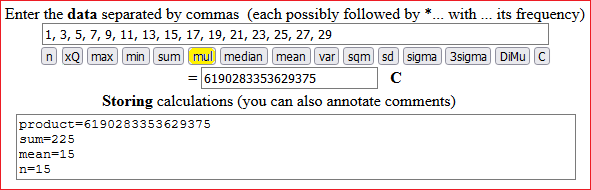
15-Fifteenth example. Use of integers
Initial sequences of positive integers can be useful for various activities. Below you can find them. An example. The sum, mean and median of the squares of the first 100 positive integers. The [N] key generates the numbers 1, 2, ..., N. We put in (g) 100 and click [N]:


If I put 2 in (j), by clicking "data^Q" I get:
1, 4, 9, 16, 25, 36, 49, 64, 81, 100, 121, 144, ..., 9604, 9801, 10000
With [copy] I copy these values into the "data" and click "sum", "mean", "median"
sum = 338350 mean=3383.5 median=2500
16-Sixteenth example. Figures displayed
The results of an operation are rounded to 17 digits but the last digit is not reliable. It is convenient (possibly using Round) to round to fewer digits, as it is necessary to do in all contexts:
asin(0.5) = 0.5235987755982989
= 30.000000000000004 ^
6 / 8 produces 0.75
0.6 / 0.8 produces 0.7499999999999999
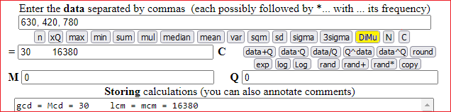
17-Seventeenth example. Greatest common divisor / Least common multiple
The [DiMu] key prints the greatest common divisor (massimo comune divisore) and least common multiple (minimo comune multiplo) of a sequence of positive integers.
18-Eighteenth example.
The order of magnitude of the results is also displayed:
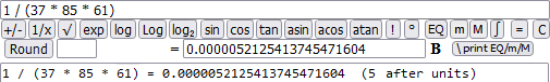
1 / (37 * 85 * 61) = 0.0000052125413745471604  (5 (after units)

pow(37 * 85 * 61, 2) = 36804504025  (11 before units)

36804504025 round to 10^ digit before units : 40000000000
                           = 0.4 * 10^11
19-Nineteenth example. Again on the use of the [ N ] key
The [N] key generates the numbers 1, 2, ..., N, which you can then transform with the [data ...] keys if you want. An example.
With [N] I generate 1, 2, ..., 20.


With 3 in [Q] and [data^Q] I get the outputs:
1, 8, 27, 64, 125, 216, 343, 512, 729, 1000, 1331, 1728, 2197, 2744, 3375, 4096, 4913, 5832, 6859, 8000
which I then copy in the box with [copy]:
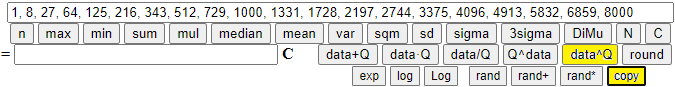
I add up these numbers:

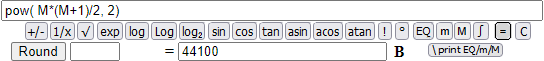
If N = 20 1³+2³+...+N³ = 44100. I verify that the same value I get with (N·(N+1)/2)².

20-Twentieth example.
•
To study how the data 5.0625,7.59375,11.390625,17.0859375,25.62890625,38.443359375 vary I can put the data in (g).
Then, if I click [log] I get the logarithm of them.
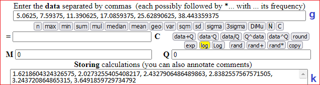
It seems to me that 1.6218604324326575, 2.0273255405408217, 2.4327906486489863, 2.8382557567571505, 3.243720864865315, 3.6491859729734792 has about the same difference. I check this with the
"repeated differences" script. I get:
0.40546510810816416,0.4054651081081646,0.40546510810816416,0.4054651081081646,0.40546510810816416
If I calculate [exp] of 0.40546510810816416 I obtain 1.4999999999999996, that is 1.5.
So starting from 5.0625 I get the other data by multiplying repeatedly by 1.5.
• If I put 1e5, 1e10, 1e20, 1e25, 1e50 in (g) and if I click [Log] I get 5, 10, 20, 25, 50.
21-Twenty-first example.
•
If in (g) I put 4000 and I click [rand] I have 4000 random numbers uniformly distributed in [0,1]. If I click
[median], [mean], [var], [sqm], [sd] I get (more or less) the following outputs:
median = 0.5093
1^,3^ quartile, diff.: 0.257 0.7573 0.5003
mean = 0.506052625
variance = 0.08317089695810909
scarto quad. medio (sq.root of var./theoret.st.dev.) = 0.288393649302666
experimental standard dev. = sqm*√(4000/3999) = 0.2884297052694635
Theoretical values:
median = 0.5
1^,3^ quartile, diff.: 0.25 0.75 0.5
mean = 0.5
variance = 1/12 = 0.08333...
scarto quad. medio (sq.root of var./theoret.st.dev.) = 1/√12 = 0.2886751345948128...
If in (g) I put 4000 and I click [rand*] I have 4000 products of 4000 pairs of random numbers uniformly distributed in [0,1]. If I click
[median], [mean], [var], [sqm], [sd] I get (more or less) the following outputs:
median = 0.1904
1^,3^ quartile, diff.: 0.0709 0.388 0.3171
mean = 0.252405
variance = 0.04844079813
scarto quad. medio (sq.root of var./theoret.st.dev.) = 0.22009270349105253
experimental standard dev. = 0.22012022023848657
22-Twenty-two example.
•
If in (g) I put some numbers and I click [geo] I have the geometric mean of them
Three machines work in series: the first has an efficiency of 89%, the second of 51%, the third of 70%. What is the overall efficiency?
68% is the overall efficiency.
23-Twenty-three example.
•
If in (g) I put some numbers and I click [arm] I have the harmonic mean of them
John trains. He travels the same road uphill at a speed of 11.6 km/h and then downhill at a speed of 16.4 km/h. What was his average speed?
24-Twenty-four example.
•
If in (d) I put a function F of the variable Q and in (a) and (b)
the endpoints of an interval [a,b] in which F changes sign, by repeatedly clicking [EQ] I find
increasingly better approximations of the solution of the equation
An example: solution of sin(x)+cos(x) = 1/2, 1 < x < 3:
I put sin(Q) + cos(Q) - 1/2 in (d), 1 in (a), 3 in (b) and repeatedly click [EQ]
25-Twenty-five example.
•
If in (d) I put a function F of the variable Q and in (a) and (b)
the endpoints of an interval [a,b] in which the graph is ∪, by repeatedly clicking [m] I find
increasingly better approximations of the abscissa of the minimum of F.
•
If in (d) I put a function F of the variable Q and in (a) and (b)
the endpoints of an interval [a,b] in which the graph is ∩, by repeatedly clicking [M] I find
increasingly better approximations of the abscissa of the maximum of F.
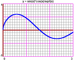
An example: max of sin(x)*cos(x)/sqrt(x), 0.1 < x < 1,
min of sin(x)*cos(x)/sqrt(x), 2 < x < 3
| sin(Q)*cos(Q)/sqrt(Q) I find max = 0.601918331 in x = 0.582780582 min = -0.327613101 in x = 2.302108378 or with more digits [ graph made by this script ] |
 |