
First example. If I click rain I have the data "mm of monthly rainfall in Genoa in the period 1984-92":
| mm mensili di pioggia a Genova nel periodo 1984-92 mm of rain per month in Genoa in the period 1984-92 41, 44, 72, 79, 197, 62, 0, 200, 52, 95, 155, 108, 71, 34, 257, 37, 161, 68, 0, 20, 14, 7, 63, 112, 172, 67, 48, 197, 16, 30, 63, 24, 115, 42, 88, 34, 70, 159, 30, 115, 65, 30, 95, 61, 88, 276, 112, 42, 187, 35, 111, 64, 101, 61, 11, 26, 25, 149, 0, 70, 10, 97, 27, 286, 12, 5, 14, 232, 57, 38, 6, 22, 34, 19, 7, 142, 2, 25, 6, 68, 61, 349, 84, 157, 44, 71, 61, 27, 93, 44, 67, 0, 423, 145, 57, 0, 47, 44, 65, 78, 16, 110, 28, 49, 391, 245, 54, 72 |
Their representation width this script, where the vertical segments are 12 (months) apart:

I want to study the presence of seasonal factors. I put the data in the first box. In the second I obtain:
In the third box I obtain: min1,max1: 0, 423 min2,max2: 10.333333333, 230 n=108
Their representation width this script:

To better smooth the trend I reapply the moving averages: I copy the output and put it in the first box using the [Copy] key. I obtain:
Their representation width this script:

I reapply the moving averages. I obtain:
Their representation width this script:

The autumn peaks are evident.
The comparison between the first and last application of moving averages, with this script.

The comparison between the data and the last application of moving averages, with this script, in which we have not represented the starting point and the final one.

If I want to get the outputs with less digits I can click [MM] again after changing the box digit after ".". If I put "3" I get the outputs rounded to 2 or 3 digits.

If I click [C] the input and output windows are cleaned.
Second example. Below are the growth rates (cm per year) of a group of North American males around 1980. We graphically represent the trend using appropriate moving averages and estimate how much the growth rate varies from the onset of puberty (minimum point, around at 10 years) to the peak value which it reaches shortly after (around 14 years). In the case of females the trend is similar, but anticipated by more than a year.
| Groth rates (cm per year) at 2, 2.5, 3, 3.5, ..., 17, 17.5 years of age Tassi di crescita (cm all'anno) all'età di 2, 2.5, 3, 3.5, ..., 17, 17.5 anni 11.6, 8.8, 7.6, 6.4, 8.4, 6.5, 6, 6.1, 7.6, 6.5, 6.3, 6.5, 5.4, 6.3, 5.2, 4.9, 4.8, 2.9, 7.4, 6.9, 5.5, 5.5, 7.6, 10.3, 9.9, 12.0, 9.4, 5.1, 5.3, 4.4, 3.7, 3.0 |
Their representation width this script, where the vertical segments are 2.5 years apart:

By calculating the moving averages three times we get:
The representation width this script:
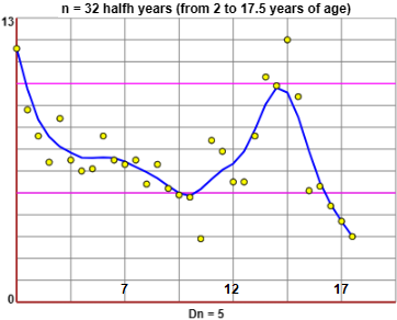
| We can estimate that, on average, the growth velocity during puberty varies from about 5 cm/year to about 10 cm/year. The "pubertal peak" (in boys around 14 years of age, in girls around 12 years of age) is regulated by particular hormones, testosterone in boys, estrogen in girls. |  |
Third example. In the graph below on the left you can see the peaks and valleys of the daily COVID case counts in a small European state, sometime in 2020. The line go up and down a lot, and usually, you will see a big peak right after a big drop. This is because not every city in the country collects and sends data every day, because, on certain days, the laboratories might not be open to report their cases, ... The graph was plotted with this script. The data:
| 213, 526, 338, 671, 429, 1182, 686, 837, 641, 783, 639, 785, 760, 613, 798, 617, 515, 631, 622, 492, 558, 398, 509, 421, 457, 568, 739, 706, 614, 742, 775, 722, 631, 643, 626, 734, 690, 787, 939, 891, 1093, 1432, 1308, 1741, 2116, 1975, 2010, 2397 |

To get a reliable chart we do the moving averages. By calculating the moving averages three times we get:
In the last step we rounded the results to 3 digits after "."
The graph on the right was plotted with this script.
Fourth example. Wholesale price in €/kg over 42 days in autumn 2010 of the copper:
On the right, the graph of this data and that of the outcome of 3 applications of the moving averages:
The graph was plotted with this script. |  |
 | On the left (see) the graph without tracing the first and last 3 points (which have not been entirely affected by the applications of the moving averages). Wholesale price in €/kg of of brass and zinc (and the moving mean):
|

Note. By repeating the procedure many times, the graph tends to become straight:

