
We can draw the graphs with JavaScript; for example, see the script Gauss (see the code; se also here).
That's the reason why the gaussian (or "normal") distribution is important:
there are a few
gaussian phenomena (see "first example"), but if I calculate the mean of N values with the same
distribution (ie if I calculate their sum divided for N), this mean has a gaussian
distribution (see "second example"). This fact goes under the name of central limit theorem:
If U1, … ,Un are random indipendent variables with the same law of distribution, and if
m and σ0 are its mean and standard deviation, when n grows the variable
The script pocket calculator-2 uses sd to indicate the standard deviation and
sigma to indicate
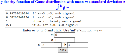
In this script I can calculate the value of the gaussian in A with mean M e sigma Q with
1/(sqrt(PI*2)*Q)*exp(-(A-M)*(A-M)/(Q*Q*2))
if I put the values of A, M and Q in the corresponding boxes.
First example, a gaussian phenomenon: the lengths of many broad beans (ie bean seeds) collected by a 12-year-old class (another example: the height of the people of a particular sex, age, place of origin). We have considered them among the examples of histogram.

n=260 min=1 max=2.3 median=1.65 mean=1.6592307692308
With pocket calculator-2 we can find the experimental standard deviation:
1*2, 1.3*2, 1.35*2, 1.4*22, 1.45*2, 1.5*24, 1.55*16, 1.6*42, 1.65*22, 1.7*42, 1.75*22, 1.8*30, 1.85*8, 1.9*16, 1.95*2, 2*2, 2.25*2, 2.3*2
n = 260 experimental standard dev. = 0.1737375439700209

We can assume that that type of beans had a Gaussian pattern of this type, with mean 1.66 and σ 0.174.
What is the probability that a bean is longer than 1.8 cm?
a ∫ b = 0.21052593458 if a = 1.8 b = inf, m = 1.66 sigma = 0.174. Rounding the value, I take 0.21 = 21%.
Second example, a non-Gaussian phenomenon: human body weight; 4170 Italian males in their twenties, in the year 1990. We have considered the file among the examples of histogram.
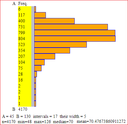
With pocket calculator-2 we can find:
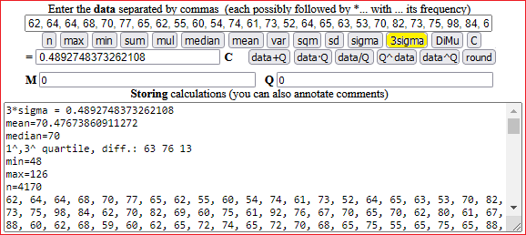
and:
experimental standard dev. = 10.531728480365418 sigma = 0.16309161244207027
The average weight (of Italian males in their twenties, in the year 1990) is 70.48±0.49 kg, or 70.5±0.5 kg.
Another example: measures (truncated to centisecond) of a period of 1 s timed by hand:
111, 103, 109, 97, 99, 110, 99, 103, 109, 106, 109, 112, 98, 110, 90, 98, 96, 90, 96, 90, 109, 103, 96, 97, 96, 96, 109, 103, 98, 94, 115, 78, 85, 96, 89, 121, 98, 103, 97, 88, 98, 129, 96, 68, 91, 80, 102
These are the values read by some people. Let's see, as an exercise, what is the duration of this time interval that we can deduce from these values.
First of all the data is truncated to the units. I have to add 1/2 in order to turn them into rounded data (I have to do this if, then, I want to consider tenths or cents!).
With pocket calculator-2:

If I then put 111.5, 103.5, 109.5, … in place of 111, 103, 109, … I have:
mean=99.86170212765957 experimental standard dev.=10.853621979931713 sigma=1.5831634778241008 3*sigma=4.749490433472302
We can say that (with practical "certainty",with a probability of 99.7%) that the true measure is 99.86 ± 3σ = 99.86 ± 4.75, or 100±5 (cs).