# I want to solve (x-2*y)^2+3*y = 4 with respect to x (fixed y=k) or y (fixed x=k)
#
# First I look for a "graphic" approximation of the solutions:
f <- function(x,y) (x-2*y)^2+3*y - 4
Plane(-3,4,-4,3)
CURVE(f,"brown")
 # Then I proceed by solving the equations numerically, first estimating from the
# graph some intervals for x, or for y, where f(x,k), or f(k,y), changes the sign:
# (I remember that solution(F,7, 1,3) solves F(x)=7 if between 1 and 3 F step across
# the value 7)
# For which x f(x,y) passes through y=0 to the left of the y axis?
h <- function(x) f(x,0); solution(h,0, -3,-1)
# -2
# For which x passes through y=1 near the y axis?
h <- function(x) f(x,1); ; solution(h,0, 0,2)
# 1
# For which y passes through x=0 under the x axis?
h <- function(y) f(0,y); solution(h,0, -2,-1)
# -1.443
#
# Finally, I check the solutions graphically:
POINT(0,-1.443,"blue"); POINT(1,1,"red"); POINT(-2,0,"black")
# Then I proceed by solving the equations numerically, first estimating from the
# graph some intervals for x, or for y, where f(x,k), or f(k,y), changes the sign:
# (I remember that solution(F,7, 1,3) solves F(x)=7 if between 1 and 3 F step across
# the value 7)
# For which x f(x,y) passes through y=0 to the left of the y axis?
h <- function(x) f(x,0); solution(h,0, -3,-1)
# -2
# For which x passes through y=1 near the y axis?
h <- function(x) f(x,1); ; solution(h,0, 0,2)
# 1
# For which y passes through x=0 under the x axis?
h <- function(y) f(0,y); solution(h,0, -2,-1)
# -1.443
#
# Finally, I check the solutions graphically:
POINT(0,-1.443,"blue"); POINT(1,1,"red"); POINT(-2,0,"black")
 #
# How to find a tangent line to a curve described as f(x,y) = 0
BF=3; HF=3
F = function(x,y) x^2+1/3*y^4-x*y-10
PLANE(-4,5, -4,5)
CURVE(F, "seagreen")
#
# How to find a tangent line to a curve described as f(x,y) = 0
BF=3; HF=3
F = function(x,y) x^2+1/3*y^4-x*y-10
PLANE(-4,5, -4,5)
CURVE(F, "seagreen")
 # The tangent line in the point that has abscissa 3 shown above
x=3 # I look for y (between 2 and 2.2)
F3=function(y) F(3,y)
y=solution(F3,0, 2,2.2)
y
# 2.181068
POINT(x,y, "red") # The point
# The tangent line has the direction of the vector: -deriv(F,"y"), deriv(F,"x")
# [ perpendicular to the vector deriv(F,"x"), deriv(F,"y") indicating the
# speed of variation in the directions of the x and y axes ]
deriv(F,"y")
# 1/3 * (4 * y^3) - x
deriv(F,"x")
# 2 * x - y
c(-(1/3 * (4 * y^3) - x), 2 * x - y)
# -10.833964 3.818932 The vector
dirArrow1(0,0, -(1/3 * (4 * y^3) - x), 2 * x - y)
# 160.5826 Its direction
# The tangent line:
point_incl(x,y, dirArrow1(0,0, -(1/3 * (4 * y^3) - x), 2 * x - y), "red")
#
# If we consider that the equation E(X,Y)=0 of the tangent line in (x,y) is
# deriv(F,"x")*(X-x) + deriv(F,"y")*(Y-y) = 0 we can also do the following:
# G = function(X,Y) (2*x-y)*(X-x)+(1/3*(4*y^3)-x)*(Y-y); CUR(G,"red")
#
# Another example:
# The tangent line to x^3+x^2*y+y^2-7*x = 0 in the point (x,1.5) with x near 2
F = function(x,y) x^3+x^2*y+y^2-7*x
BF=3; HF=3; PLANE(-8,8, -8,8); CURVE(F, "brown")
abline(h=1.5,col="red"); text(7,2.5,"y=1.5")
# The tangent line in the point that has abscissa 3 shown above
x=3 # I look for y (between 2 and 2.2)
F3=function(y) F(3,y)
y=solution(F3,0, 2,2.2)
y
# 2.181068
POINT(x,y, "red") # The point
# The tangent line has the direction of the vector: -deriv(F,"y"), deriv(F,"x")
# [ perpendicular to the vector deriv(F,"x"), deriv(F,"y") indicating the
# speed of variation in the directions of the x and y axes ]
deriv(F,"y")
# 1/3 * (4 * y^3) - x
deriv(F,"x")
# 2 * x - y
c(-(1/3 * (4 * y^3) - x), 2 * x - y)
# -10.833964 3.818932 The vector
dirArrow1(0,0, -(1/3 * (4 * y^3) - x), 2 * x - y)
# 160.5826 Its direction
# The tangent line:
point_incl(x,y, dirArrow1(0,0, -(1/3 * (4 * y^3) - x), 2 * x - y), "red")
#
# If we consider that the equation E(X,Y)=0 of the tangent line in (x,y) is
# deriv(F,"x")*(X-x) + deriv(F,"y")*(Y-y) = 0 we can also do the following:
# G = function(X,Y) (2*x-y)*(X-x)+(1/3*(4*y^3)-x)*(Y-y); CUR(G,"red")
#
# Another example:
# The tangent line to x^3+x^2*y+y^2-7*x = 0 in the point (x,1.5) with x near 2
F = function(x,y) x^3+x^2*y+y^2-7*x
BF=3; HF=3; PLANE(-8,8, -8,8); CURVE(F, "brown")
abline(h=1.5,col="red"); text(7,2.5,"y=1.5")
 G = function(x) F(x,1.5); x=solution(G,0, 1,3); y=1.5; x
# 1.756267
POINT(x,y, "black")
# The tangent line has the direction -deriv(F,"y"), deriv(F,"x")
deriv(F,"x")
# 3 * x^2 + 2 * x * y - 7
deriv(F,"y")
# x^2 + 2 * y
d = dirArrow1(0,0, -(x^2 + 2 * y),3 * x^2 + 2 * x * y - 7); d
# 128.9682
point_inclina(x,y, d, "blue")
#
# If we consider that the equation E(X,Y)=0 of the tangent line in (x,y) is
# deriv(F,"x")*(X-x) + deriv(F,"y")*(Y-y) = 0 we can also do the following:
# H = function(X,Y) (3*x^2+2*x*y-7)*(X-x)+(x^2+2*y)*(Y-y); CUR(H,"blue")
#
# Another problem:
# the parabola that is tangent to x = 2 in (2,0) and to y = 1 in (0,1)
G = function(x) F(x,1.5); x=solution(G,0, 1,3); y=1.5; x
# 1.756267
POINT(x,y, "black")
# The tangent line has the direction -deriv(F,"y"), deriv(F,"x")
deriv(F,"x")
# 3 * x^2 + 2 * x * y - 7
deriv(F,"y")
# x^2 + 2 * y
d = dirArrow1(0,0, -(x^2 + 2 * y),3 * x^2 + 2 * x * y - 7); d
# 128.9682
point_inclina(x,y, d, "blue")
#
# If we consider that the equation E(X,Y)=0 of the tangent line in (x,y) is
# deriv(F,"x")*(X-x) + deriv(F,"y")*(Y-y) = 0 we can also do the following:
# H = function(X,Y) (3*x^2+2*x*y-7)*(X-x)+(x^2+2*y)*(Y-y); CUR(H,"blue")
#
# Another problem:
# the parabola that is tangent to x = 2 in (2,0) and to y = 1 in (0,1)
 BF=3; HF=3; PLANE(-4,4, -4,4)
abline(h=1, col="red"); abline(v=2, col="red"); POINT(2,0,"red"); POINT(0,1, "red")
# A generic conic:
W = function(x,y) a*x^2 + b*x*y + c*y^2 + d*x + e*y + f
# For a parabola we have b^2=4ac, or c=b^2/(4a); we can put a=1
a = 1; c = b^2/4
# I passes through (0,1) and (2,0): b^2/4+e+f=0, 4+2d+f=0 -> b^2/4+e=2*d+4
# The tangent line has the direction -deriv(F,"y"), deriv(F,"x")
# deriv(F,"x") = 2*x+b*y+d; deriv(F,"y") = b*x+b^2*y+e
# in (0,1) deriv(F,"x") = b+d must be 0 -> d=-b
# in (2,0) deriv(F,"y") = 2*b+e must be 0 -> e=-2*b
# f = -4+2*b; b^2/4+e=2*d+4 -> b^2 = 16 If I put:
b = -4; a =1; c = b^2/4; d = -b; e = -2*b; f = -4+2*b
CURV(W, "brown")
c(a,b,c,d,e,f)
# 1 -4 4 4 8 -12
# With b = 4 I have a degenerate conic: the null set.
#
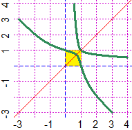
# Another problem: to study the curve 2^(x*y) = x+y
BF=3; HF=3; PLANE(-3,4, -3,4)
H = function(x,y) 2^(x*y)-x-y
CURVE(H, "seagreen"); abline(0,1, col="red")
# Or (incorporating y = x), to have a thin-stroke:
K = function(x,y) H(x,y)*(y-x)
a=-3; b=4; PLANE(a,b, a,b); CUR(K, "brown")
BF=3; HF=3; PLANE(-4,4, -4,4)
abline(h=1, col="red"); abline(v=2, col="red"); POINT(2,0,"red"); POINT(0,1, "red")
# A generic conic:
W = function(x,y) a*x^2 + b*x*y + c*y^2 + d*x + e*y + f
# For a parabola we have b^2=4ac, or c=b^2/(4a); we can put a=1
a = 1; c = b^2/4
# I passes through (0,1) and (2,0): b^2/4+e+f=0, 4+2d+f=0 -> b^2/4+e=2*d+4
# The tangent line has the direction -deriv(F,"y"), deriv(F,"x")
# deriv(F,"x") = 2*x+b*y+d; deriv(F,"y") = b*x+b^2*y+e
# in (0,1) deriv(F,"x") = b+d must be 0 -> d=-b
# in (2,0) deriv(F,"y") = 2*b+e must be 0 -> e=-2*b
# f = -4+2*b; b^2/4+e=2*d+4 -> b^2 = 16 If I put:
b = -4; a =1; c = b^2/4; d = -b; e = -2*b; f = -4+2*b
CURV(W, "brown")
c(a,b,c,d,e,f)
# 1 -4 4 4 8 -12
# With b = 4 I have a degenerate conic: the null set.
#
# Another problem: to study the curve 2^(x*y) = x+y
BF=3; HF=3; PLANE(-3,4, -3,4)
H = function(x,y) 2^(x*y)-x-y
CURVE(H, "seagreen"); abline(0,1, col="red")
# Or (incorporating y = x), to have a thin-stroke:
K = function(x,y) H(x,y)*(y-x)
a=-3; b=4; PLANE(a,b, a,b); CUR(K, "brown")
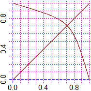
 # To find the "maximum curvature" points I can simply do some zooming
# The first is evidently (1,1) [H(1,1)=0]. The point in [0,1)×[0,1):
a=0; b=1; PLANE(a,b, a,b); CUR(K,"brown")
# ...
a=0.7071065; b=0.707107; PLANE(a,b, a,b); CUR(K, "brown")
# To find the "maximum curvature" points I can simply do some zooming
# The first is evidently (1,1) [H(1,1)=0]. The point in [0,1)×[0,1):
a=0; b=1; PLANE(a,b, a,b); CUR(K,"brown")
# ...
a=0.7071065; b=0.707107; PLANE(a,b, a,b); CUR(K, "brown")
 # It makes no sense to proceed with further zooming. After all:
a=0.7071068; b=a; H(a,b)
# -1.154592e-08 near 0
# "a" is a known number?
a^2
# 0.5 So a = b = 1/sqrt(2) = 2^(-1/2)
# Can we find the solution in other way? Study this problem!
#
# A curve with a node: y*(y-2*x)-x^3 = 0
F = function(x,y) y*(y-2*x)-x^3
BF=3; HF=3; PLANE(-2,3, -2,3)
CURVE(F, "seagreen")
# It makes no sense to proceed with further zooming. After all:
a=0.7071068; b=a; H(a,b)
# -1.154592e-08 near 0
# "a" is a known number?
a^2
# 0.5 So a = b = 1/sqrt(2) = 2^(-1/2)
# Can we find the solution in other way? Study this problem!
#
# A curve with a node: y*(y-2*x)-x^3 = 0
F = function(x,y) y*(y-2*x)-x^3
BF=3; HF=3; PLANE(-2,3, -2,3)
CURVE(F, "seagreen")

 # With some zoom I can guess that the curve passes through points (0,0) and
# (-1,-1). And in fact F(0,0) = 0, F(-1,-1) = 0.
# The tangent line has the direction of the vector: -deriv(F,"y"), deriv(F,"x")
# [ perpendicular to the vector deriv(F,"x"), deriv(F,"y") indicating the
# speed of variation in the directions of the x and y axes ]
# The tangent line in (-1,-1):
deriv(F,"x"); deriv(F,"y")
# -(y * 2 + 3 * x^2) (y - 2 * x) + y
x = -1; y = -1; c( -(y-2*x)-y, -(y*2+3*x^2) )
# 0 -1
# In (-1,-1) the tangent line is direct as (0,-1): it's vertical
# That is, it's (-1)*(X+1)+0*(Y-0) = 0; that is X = -1
# In (0,0) there is a node. It is a double point. There are two tangents
# depending on how you move. I can't find them with the previous equation
# (which would become 0 = 0).
# It can be shown that if in (0,0) there is such a situation, the two
# tangents are describable with A*x^2+B*x*y+C*y^2 = 0 if F(x,y) is the
# polynomial A*x^2+B*x*y+C*y^2+... In our case, A=0, B=-2, C=1: y(y-2x)=0.
# The two tangents in (0,0) are y=0 and y=2*x.
# In the case of the third point, how do we proceed?
# I know that his abscissa is between -1 and -1/2.
# The tangent line has the direction of the vector: -deriv(F,"y"), deriv(F,"x")
# I have to look (x,y) that is on the curve and where deriv(F,"x")=0
# y*(y-2*x)-x^3=0, y*2 + 3*x^2=0
# y*(y-2*x)-x^3=0, y = -3*x^2/2
h = function(x) -3*x^2/2*(-3*x^2/2-2*x)-x^3
q = solution(h,0, -1,-1/2); q; fraction(q)
# -0.8888889 -8/9
# I look for the ordinate (between -1.3 and -1)
W = function(y) F(-8/9,y)
qq = solution(W,0, -1.3,-1); qq; fraction(qq)
# -1.185185 -32/27
# The point is (-8/9, -32/27)
POINT(0,0, "brown"); POINT(-1,-1, "brown"); POINT(-8/9,-32/27, "brown")
f = function(x) 2*x
graph1(f, -2,3, "brown")
#
# A curve with a cusp (or with a corner?): (x-y^2)^2-y^5 = 0
# (a point with the same tangent line or with two different tangent lines?)
F = function(x,y) (x-y^2)^2-y^5
BF=3; HF=3; PLANE(-2,3, -2,3)
CURVE(F, "seagreen")
# With some zoom I can guess that the curve passes through points (0,0) and
# (-1,-1). And in fact F(0,0) = 0, F(-1,-1) = 0.
# The tangent line has the direction of the vector: -deriv(F,"y"), deriv(F,"x")
# [ perpendicular to the vector deriv(F,"x"), deriv(F,"y") indicating the
# speed of variation in the directions of the x and y axes ]
# The tangent line in (-1,-1):
deriv(F,"x"); deriv(F,"y")
# -(y * 2 + 3 * x^2) (y - 2 * x) + y
x = -1; y = -1; c( -(y-2*x)-y, -(y*2+3*x^2) )
# 0 -1
# In (-1,-1) the tangent line is direct as (0,-1): it's vertical
# That is, it's (-1)*(X+1)+0*(Y-0) = 0; that is X = -1
# In (0,0) there is a node. It is a double point. There are two tangents
# depending on how you move. I can't find them with the previous equation
# (which would become 0 = 0).
# It can be shown that if in (0,0) there is such a situation, the two
# tangents are describable with A*x^2+B*x*y+C*y^2 = 0 if F(x,y) is the
# polynomial A*x^2+B*x*y+C*y^2+... In our case, A=0, B=-2, C=1: y(y-2x)=0.
# The two tangents in (0,0) are y=0 and y=2*x.
# In the case of the third point, how do we proceed?
# I know that his abscissa is between -1 and -1/2.
# The tangent line has the direction of the vector: -deriv(F,"y"), deriv(F,"x")
# I have to look (x,y) that is on the curve and where deriv(F,"x")=0
# y*(y-2*x)-x^3=0, y*2 + 3*x^2=0
# y*(y-2*x)-x^3=0, y = -3*x^2/2
h = function(x) -3*x^2/2*(-3*x^2/2-2*x)-x^3
q = solution(h,0, -1,-1/2); q; fraction(q)
# -0.8888889 -8/9
# I look for the ordinate (between -1.3 and -1)
W = function(y) F(-8/9,y)
qq = solution(W,0, -1.3,-1); qq; fraction(qq)
# -1.185185 -32/27
# The point is (-8/9, -32/27)
POINT(0,0, "brown"); POINT(-1,-1, "brown"); POINT(-8/9,-32/27, "brown")
f = function(x) 2*x
graph1(f, -2,3, "brown")
#
# A curve with a cusp (or with a corner?): (x-y^2)^2-y^5 = 0
# (a point with the same tangent line or with two different tangent lines?)
F = function(x,y) (x-y^2)^2-y^5
BF=3; HF=3; PLANE(-2,3, -2,3)
CURVE(F, "seagreen")
 F(0,0) # 0
POINT(0,0, "brown")
F(0,1) # 0
POINT(0,1, "brown")
F(2,1) # 0
POINT(2,1, "brown")
k = function(x) F(x,2)
yy=solution(k,0, -2, -1); yy # -1.656854
POINT(yy,2,"brown")
u = function(y) F(1,y)
yy = solution(u,0, 1/2, 1); yy # 0.7338919
POINT(1,yy,"brown")
# Let's zoom in to see what happens in (0,0)
PLANE(-0.5,0.0, 0,1); CURVE(F, "seagreen")
PLANE(-0.2,0.2, 0,0.4); CURVE(F, "seagreen")
F(0,0) # 0
POINT(0,0, "brown")
F(0,1) # 0
POINT(0,1, "brown")
F(2,1) # 0
POINT(2,1, "brown")
k = function(x) F(x,2)
yy=solution(k,0, -2, -1); yy # -1.656854
POINT(yy,2,"brown")
u = function(y) F(1,y)
yy = solution(u,0, 1/2, 1); yy # 0.7338919
POINT(1,yy,"brown")
# Let's zoom in to see what happens in (0,0)
PLANE(-0.5,0.0, 0,1); CURVE(F, "seagreen")
PLANE(-0.2,0.2, 0,0.4); CURVE(F, "seagreen")
 # After the zooms, there seems to be a cusp.
deriv(F,"x"); deriv(F,"y")
# 2 * (x - y^2) -(2 * (2 * y * (x - y^2)) + 5 * y^4)
# In (0,0) the two partial derivatives are 0, as in the previous case of the node.
# It can be shown that if in (0,0) there is such a situation, the tangent line
# is describable with A*x^2+B*x*y+C*y^2 = 0 if F(x,y) is the
# polynomial A*x^2+B*x*y+C*y^2+... In our case, A=1, B=0, C=0.
# The tangent line in (0,0) is x=0.
# After the zooms, there seems to be a cusp.
deriv(F,"x"); deriv(F,"y")
# 2 * (x - y^2) -(2 * (2 * y * (x - y^2)) + 5 * y^4)
# In (0,0) the two partial derivatives are 0, as in the previous case of the node.
# It can be shown that if in (0,0) there is such a situation, the tangent line
# is describable with A*x^2+B*x*y+C*y^2 = 0 if F(x,y) is the
# polynomial A*x^2+B*x*y+C*y^2+... In our case, A=1, B=0, C=0.
# The tangent line in (0,0) is x=0.
