Un procedimento decisamente sbagliato, che non tiene conto che la retta deve passare per (0,0):
A decidedly wrong procedure, which does not take into account that the line must pass through (0,0):

|
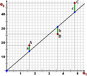
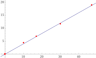
Here's how you can go about it. In three experiments I obtain the pairs (G1,G2) represented on the side with the points A, B and C. I search, among all the graphs of the type a = |yA - k xA|, b = |yB - k xB|, c = |yC - k xC| a²+ b²+ c² = (k xA - yA)²+ (k xB - yB)²+ (k xC - yC)². It is a polynomial expression in k of the second degree. It has a minimum value when its derivative with respect to k is canceled, that is when: 2(k xA - yA)xA + 2(k xB - yB)xB + 2(k xC - yC)xC = 0 i.e. k = (xAyA+ xByB+ xCyC)/(xA² + xB² + xC²). If I had imposed that the line passed through (p,q) instead of O, I could have performed a similar calculation obtaining: k = ( (xA-p)(yA-q)+(xB-p)(yB-q)+(xC-p)(yC-q) ) / ( (xA-p)² +(xB-p)² + (xC-p)² ). |
Torniamo al problema iniziale / Let's go back to the initial problem

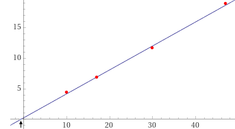
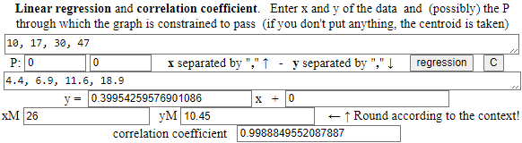
( 10*4.4+17*6.9+30*11.6+47*18.9 ) / ( 10^2+17^2+30^2+47^2 )
0.3995425957...
y = 0.3995 x
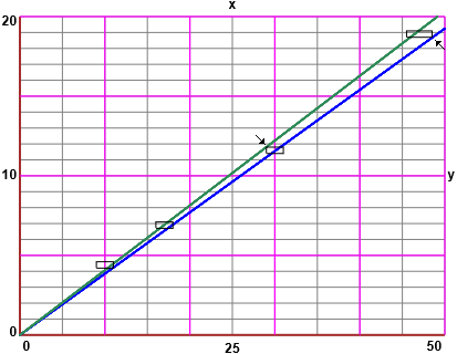
Ma potrei usare un semplice script / But I could use a simple script (vedi/see)
Per fare il grafico con "linear fit" posso aggiungere un po' di punti fissi / To make the graph with "linear fit" I can add some fixed points

{(10,4.4),(17,6.9),(30,11.6),(47,18.9), (0,0),(0,0),(0,0),(0,0),(0,0),(0,0),(0,0),(0,0),(0,0),(0,0),(0,0),(0,0),(0,0),(0,0),(0,0),(0,0),(0,0),(0,0),(0,0),(0,0)}
Ma anche procedendo così non ho tenuto conto delle precisioni / But even proceeding in this way, I did not take into account the uncertainties
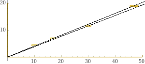
La corretta soluzione, trovata graficamente / The correct solution, found graphically
La retta di minima pendenza passa per (47+1.5,18.9-0.2); 18.7/48.5 = 0.38556… Quella di massima pendenza per (30-1,11.6+0.2); 11.8/29 = 0.40689…
The line of minimum slope passes through (47+1.5,18.9-0.2); 18.7/48.5 = 0.38556… That of maximum slope through (30-1,11.6+0.2); 11.8/29 = 0.40689…
Come potremmo fare il grafico con / How could we chart with WolframAlpha:
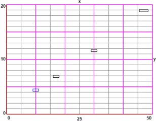
rectangle (0,0),(50,0),(50,20),(0,20), rectangle (47-1.5,18.9-0.2),(47-1.5,18.9+0.2),(47+1.5,18.9+0.2),(47+1.5,18.9-0.2)
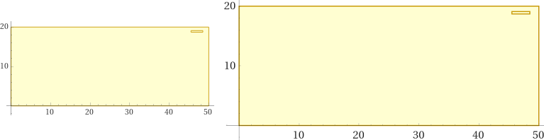
Abbiamo tracciato un punto, con l'immagine che può essere (ingrandita e poi) copiata in Paint o in un'altra applicazione grafica.
We have drawn a point, with the image that can be (enlarged and then) copied into Paint or another graphics application.

Posso colorare bianca la base del grafico, tracciare i grafici degli altri punti e incollarli in trasparenza sul primo grafico.
I can paint the base of the graph white, draw the graphs of the other points and paste them transparently on the first graph.
rectangle (0,0),(50,0),(50,20),(0,20), rectangle (30-1,11.6-0.2),(30-1,11.6+0.2),(30+1,11.6+0.2),(30+1,11.6-0.2)
rectangle (0,0),(50,0),(50,20),(0,20), rectangle (17-1,6.9-0.2),(17-1,6.9+0.2),(17+1,6.9+0.2),(17+1,6.9-0.2)
rectangle (0,0),(50,0),(50,20),(0,20), rectangle (10-1,4.4-0.2),(10-1,4.4+0.2),(10+1,4.4+0.2),(10+1,4.4-0.2)
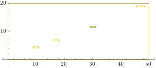
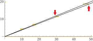
Poi posso colorare di bianco il bordo e trovare graficamente le rette di minima e massima pendenza.
Then I can color the edge white and graphically find the lines of minimum and maximum slope.
Senza utilizzare il grafico potremmo fare i calcoli con / Without using the graph we could do the calculations with WolframAlpha:
max {(4.4-0.2)/(10+1), (6.9-0.2)/(17+1), (11.6-0.2)/(30+1), (18.9-0.2)/(47+1.5)}
0.385567
min {(4.4+0.2)/(10-1), (6.9+0.2)/(17-1), (11.6+0.2)/(30-1), (18.9+0.2)/(47-1.5)}
0.406897
Posso dedurre che y/x varia tra 0.38 e 0.41 / I can deduce that y/x varies between 0.38 and 0.41
La retta di minima pendenza passa per (47+1.5,18.9-0.2); 18.7/48.5 = 0.38556… ≥ 0.38. Quella di massima pendenza per (30-1,11.6+0.2); 11.8/29 = 0.40689… ≤ 0.41.
La retta di minima pendenza passa per (47+1.5,18.9-0.2); 18.7/48.5 = 0.38556… ≥ 0.38. Quella di massima pendenza per (30-1,11.6+0.2); 11.8/29 = 0.40689… ≤ 0.41.
Senza utilizzare il grafico potremmo fare i calcoli con WolframAlpha:
max {(4.4-0.2)/(10+1), (6.9-0.2)/(17+1), (11.6-0.2)/(30+1), (18.9-0.2)/(47+1.5)}
0.385567
min {(4.4+0.2)/(10-1), (6.9+0.2)/(17-1), (11.6+0.2)/(30-1), (18.9+0.2)/(47-1.5)}
0.406897
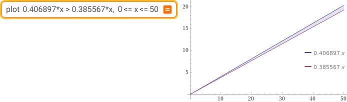
plot 0.406897*x > 0.385567*x, 0 <= x <= 50
Posso dedurre che y/x varia tra 0.38 e 0.41 / I can deduce that y/x varies between 0.38 and 0.41
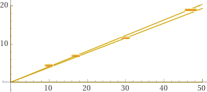
Se volessi potrei tracciare le rette sulla stessa scala e sovrapporre ad esse il grafico precedente
If I wanted to, I could draw the lines on the same scale and superimpose the previous graph on them
rectangle (0,0),(50,0),(50,20),(0,20), rectangle (0,0),(50,50*0.406897),(50,50*0.406897),(0,0), rectangle (0,0),(50,50*0.385567),(50,50*0.385567),(0,0)
Qui/here il grafico in JavaScript