source("http://macosa.dima.unige.it/r.R") # If I have not already loaded the library
# experimental points that I know have polynomial behavior
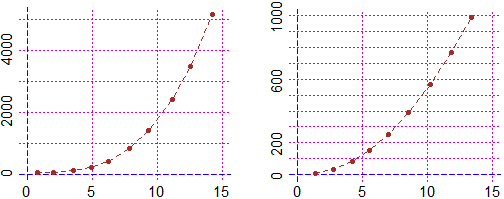
x = c(0.8, 2, 3.5,4.9, 6.2, 7.8, 9.3, 11.1,12.5,14.2)
y = c(54.104,59,104,218.3,416.3,821.6,1404,2421,3493,5177)
BF=3.5; HF=2.5
Plane(0,15, 50,5200)
Point(x,y,"brown"); polyli(x,y,"brown")
# I draw the graph of the slope (I take the value at the center
# of each interval)
length(x)
# 10 (they are 10 points)
n = 1:(length(x)-1)
dy = (y[n+1]-y[n])/(x[n+1]-x[n]); dx = (x[n+1]+x[n])/2
# I calculate in which range the slope varies
min(dy); max(dy)
# 4.08 990.5882
# I memorize the previous graph, because then I'll call it
fig = recordPlot()
Plane(0,15, 0,1000)
Point(dx,dy,"brown"); polyli(dx,dy,"brown")
 # I draw the graph of the slope of the slope
n = 1:(length(Px)-2)
ddy = (dy[n+1]-dy[n])/(dx[n+1]-dx[n]); ddx = (dx[n+1]+dx[n])/2
min(ddy); max(ddy)
# 19.2 145.08
Plane(0,15, 0,150)
Point(ddx,ddy,"brown"); polyli(ddx,ddy,"brown")
# With 2 steps to the slope I arrive at a (almost) linear trend; therefore the
# tabulated function was a polynomial of degree 3
# I draw the graph of the slope of the slope of the slope
n = 1:(length(Px)-3)
dddy = (ddy[n+1]-ddy[n])/(ddx[n+1]-ddx[n]); dddx = (ddx[n+1]+ddx[n])/2
min(dddy); max(dddy)
# 11.28327 12.52744
Plane(0,15, 0,14)
Point(dddx,dddy,"brown"); polyli(dddx,dddy,"brown")
# I draw the graph of the slope of the slope
n = 1:(length(Px)-2)
ddy = (dy[n+1]-dy[n])/(dx[n+1]-dx[n]); ddx = (dx[n+1]+dx[n])/2
min(ddy); max(ddy)
# 19.2 145.08
Plane(0,15, 0,150)
Point(ddx,ddy,"brown"); polyli(ddx,ddy,"brown")
# With 2 steps to the slope I arrive at a (almost) linear trend; therefore the
# tabulated function was a polynomial of degree 3
# I draw the graph of the slope of the slope of the slope
n = 1:(length(Px)-3)
dddy = (ddy[n+1]-ddy[n])/(ddx[n+1]-ddx[n]); dddx = (ddx[n+1]+ddx[n])/2
min(dddy); max(dddy)
# 11.28327 12.52744
Plane(0,15, 0,14)
Point(dddx,dddy,"brown"); polyli(dddx,dddy,"brown")
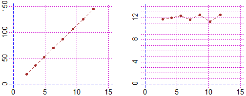 # From the fact that the last graph is, approximately, the straight line of ordinate 12 I
# deduce that the leading coefficient of the polynomial is, approximately, 12/3/2 = 2
#
# We verify what we have found by searching directly (with the cubic regression) for
# the 3rd degree polynomial that best approximates the initial data
regression3(x,y)
# 2 * x^3 + -2.99 * x^2 + -0.0629 * x + 55.1
f = function(x) 2 * x^3 + -2.99 * x^2 + -0.0629 * x + 55.1
# Let's try to superimpose the graph of f on the initial points
replayPlot(fig)
graph1(f, 0,15, "blue")
# From the fact that the last graph is, approximately, the straight line of ordinate 12 I
# deduce that the leading coefficient of the polynomial is, approximately, 12/3/2 = 2
#
# We verify what we have found by searching directly (with the cubic regression) for
# the 3rd degree polynomial that best approximates the initial data
regression3(x,y)
# 2 * x^3 + -2.99 * x^2 + -0.0629 * x + 55.1
f = function(x) 2 * x^3 + -2.99 * x^2 + -0.0629 * x + 55.1
# Let's try to superimpose the graph of f on the initial points
replayPlot(fig)
graph1(f, 0,15, "blue")
 # OK
# OK