source("http://macosa.dima.unige.it/r.R") # <- If I have not already loaded the library
# If I have the points that have the following coordinates: bilog.htm and I know that
# they are of the graph of a polynomial function, I can find the degree of it if I
# transform x and y coordinates by the logarithmic function. I can copy the file to the
# clipboard and then with
dati = read.table("clipboard",sep=",")
dim(dati)
# 21 2
x=dati$V1; y=dati$V2
min(x); max(x); min(y); max(y)
# -1 15 1.215313e-10 6080
BF=4; HF=3
Plane(-1,15, 0,6100)
Point(x,y, "blue")
# I have the graph below left
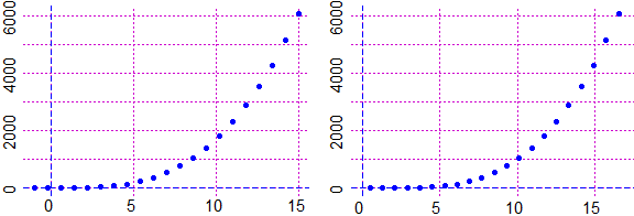 # To transform the data with the logarithmic scales, I add two constants in order to
# obtain positive coordinates.
x1=x+1.5; y1=y+1
min(x1); max(x1); min(y1); max(y1)
# 0.5 16.5 1 6081
Plane(0,17, 0,6100); Point(x1,y1, "blue")
# Having obtained the graph on the right, I transform it using logarithmic function.
x2=log(x1); y2=log(y1)
min(x2); max(x2); min(y2); max(y2)
# -0.6931472 2.80336 1.2153e-10 8.712924
Plane(-1,3, 0,9); Point(x2,y2, "blue")
# I get the graph below left:
# To transform the data with the logarithmic scales, I add two constants in order to
# obtain positive coordinates.
x1=x+1.5; y1=y+1
min(x1); max(x1); min(y1); max(y1)
# 0.5 16.5 1 6081
Plane(0,17, 0,6100); Point(x1,y1, "blue")
# Having obtained the graph on the right, I transform it using logarithmic function.
x2=log(x1); y2=log(y1)
min(x2); max(x2); min(y2); max(y2)
# -0.6931472 2.80336 1.2153e-10 8.712924
Plane(-1,3, 0,9); Point(x2,y2, "blue")
# I get the graph below left:
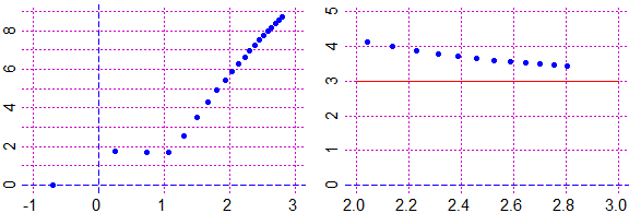 # I understand that the function tends to have slope 3, ie that the polynomial
# function has degree 3. I can verify this by calculating the slopes:
for(i in 1:20) print((y2[i+1]-y2[i])/(x2[i+1]-x2[i]))
# 1.851189 ... 3.520021 3.486567 3.457125 3.431019
# I can also represent this graphically (see above right):
Plane(2,3, 0,5)
for(i in 5:20) Point(x2[i+1], (y2[i+1]-y2[i])/(x2[i+1]-x2[i]), "blue")
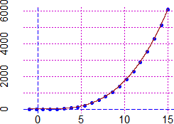
# Now I can find the function with "regression3" (see here):
regression3(x,y)
# 2 * x^3 + -3 * x^2 + -1.76e-11 * x + 5
f = function(x) 2 * x^3 - 3 * x^2 + 5
Plane(-1,15, 0,6100); Point(x,y, "blue")
graph1(f, -1,15, "brown")
# I get the graph:
# I understand that the function tends to have slope 3, ie that the polynomial
# function has degree 3. I can verify this by calculating the slopes:
for(i in 1:20) print((y2[i+1]-y2[i])/(x2[i+1]-x2[i]))
# 1.851189 ... 3.520021 3.486567 3.457125 3.431019
# I can also represent this graphically (see above right):
Plane(2,3, 0,5)
for(i in 5:20) Point(x2[i+1], (y2[i+1]-y2[i])/(x2[i+1]-x2[i]), "blue")
# Now I can find the function with "regression3" (see here):
regression3(x,y)
# 2 * x^3 + -3 * x^2 + -1.76e-11 * x + 5
f = function(x) 2 * x^3 - 3 * x^2 + 5
Plane(-1,15, 0,6100); Point(x,y, "blue")
graph1(f, -1,15, "brown")
# I get the graph: