Integrazione definita con R e controllo della indefinita
## Calcoli introdotti QUI.
#
# source("http://macosa.dima.unige.it/r.R")
f = function(x) sqrt(1-x*x); integral(f, -1,1)
## 1.570796
# Vediamo come ottenere più cifre:
more( integral(f, -1,1) )
## 1.5707963267949
# Confrontiamolo con π/2:
more( pi/2 )
## 1.5707963267949 OK!
#
# Altri integrali:
f = function(x) x^3+2; graphF(f, -2,2, "brown"); POINT(0,2, "red")
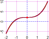 integral(f ,-2,2)
## 8
#
f = function(x) 1/x; integral(f,1,3); more(integral(f, 1,3))
1.098612 1.09861228866811
more( log(3) )
## 1.09861228866811
#
## Calcoli introdotti QUI.
#
# Controllo che l'integrale di excos(x) sia ex(cos(x)+sin(x))/2 (+C)
f = function(x) exp(x)*(cos(x)+sin(x))/2; deriv(f, "x")
## (exp(x)*(cos(x)+sin(x))+exp(x)*(cos(x)-sin(x)))/2
# Verifica "grafica" che coincida con excos(x)
df <- function(x) eval(deriv(f,"x")); graphF(df,-5,5, "red")
k = function(x) exp(x)*cos(x); graph1(k, -5,5, "black")
integral(f ,-2,2)
## 8
#
f = function(x) 1/x; integral(f,1,3); more(integral(f, 1,3))
1.098612 1.09861228866811
more( log(3) )
## 1.09861228866811
#
## Calcoli introdotti QUI.
#
# Controllo che l'integrale di excos(x) sia ex(cos(x)+sin(x))/2 (+C)
f = function(x) exp(x)*(cos(x)+sin(x))/2; deriv(f, "x")
## (exp(x)*(cos(x)+sin(x))+exp(x)*(cos(x)-sin(x)))/2
# Verifica "grafica" che coincida con excos(x)
df <- function(x) eval(deriv(f,"x")); graphF(df,-5,5, "red")
k = function(x) exp(x)*cos(x); graph1(k, -5,5, "black")
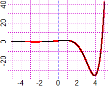 # Si sovrappone: OK
#
f = function(x) atan(x); integral(f, 0,1); more(integral(f, 0,1))
## 0.4388246 0.438824573117476
more( pi/4-log(2)/2 )
## 0.438824573117476
#
# - - - - - - - - - - - - - - - - - - - - - - - - - - - - - - - -
#
# Senza caricare il file "http://macosa.dima.unige.it/r.R"
#
# Calcoliamo l'integrale tra -1 ed 1 della seguente funzione:
f = function(x) sqrt(1-x*x)
integrate(f,-1,1)
# Ecco cosa ottengo
1.570796 with absolute error < 1e-09
# Se voglio solo il valore dell'integrale batto:
integrate(f,-1,1)$value
1.570796
# È il valore di π/2. Vediamo come ottenere più cifre:
library(codetools)
showTree(integrate(f,-1,1)$value)
1.57079632679490
# Senza caricare codetools potevo procedere (qui e nel seguito)
# con
print(integrate(f,-1,1),16)
1.570796326794898 with absolute error < 1e-09
# o con print(integrate(f,-1,1)$value,16)
# Confrontiamolo con π/2:
showTree(pi/2)
1.57079632679490
# OK
#
# Altri integrali:
f = function(x) x^3+2
plot(f,-2,2); abline(h=0,v=0,col="blue")
# Si sovrappone: OK
#
f = function(x) atan(x); integral(f, 0,1); more(integral(f, 0,1))
## 0.4388246 0.438824573117476
more( pi/4-log(2)/2 )
## 0.438824573117476
#
# - - - - - - - - - - - - - - - - - - - - - - - - - - - - - - - -
#
# Senza caricare il file "http://macosa.dima.unige.it/r.R"
#
# Calcoliamo l'integrale tra -1 ed 1 della seguente funzione:
f = function(x) sqrt(1-x*x)
integrate(f,-1,1)
# Ecco cosa ottengo
1.570796 with absolute error < 1e-09
# Se voglio solo il valore dell'integrale batto:
integrate(f,-1,1)$value
1.570796
# È il valore di π/2. Vediamo come ottenere più cifre:
library(codetools)
showTree(integrate(f,-1,1)$value)
1.57079632679490
# Senza caricare codetools potevo procedere (qui e nel seguito)
# con
print(integrate(f,-1,1),16)
1.570796326794898 with absolute error < 1e-09
# o con print(integrate(f,-1,1)$value,16)
# Confrontiamolo con π/2:
showTree(pi/2)
1.57079632679490
# OK
#
# Altri integrali:
f = function(x) x^3+2
plot(f,-2,2); abline(h=0,v=0,col="blue")
 integrate(f,-2,2)
8 with absolute error < 1.3e-13
#
f = function(x) 1/x
integrate(f,1,3)
1.098612 with absolute error < 7.6e-14
showTree(integrate(f,1,3)$value)
1.09861228866811
showTree(log(3))
1.09861228866811
#
## Calcoli introdotti QUI.
#
# Controllo che l'integrale di excos(x) sia ex(cos(x)+sin(x))/2 (+C)
D(expression(exp(x)*(cos(x)+sin(x))/2), "x")
(exp(x)*(cos(x)+sin(x))+exp(x)*(cos(x)-sin(x)))/2
# Verifica "grafica" che coincida con excos(x)
h = function(x) (exp(x)*(cos(x)+sin(x))+exp(x)*(cos(x)-sin(x)))/2
plot(h,-5,5)
k = function(x) exp(x)*cos(x)
plot(k,-5,5,add=TRUE,col="blue")
integrate(f,-2,2)
8 with absolute error < 1.3e-13
#
f = function(x) 1/x
integrate(f,1,3)
1.098612 with absolute error < 7.6e-14
showTree(integrate(f,1,3)$value)
1.09861228866811
showTree(log(3))
1.09861228866811
#
## Calcoli introdotti QUI.
#
# Controllo che l'integrale di excos(x) sia ex(cos(x)+sin(x))/2 (+C)
D(expression(exp(x)*(cos(x)+sin(x))/2), "x")
(exp(x)*(cos(x)+sin(x))+exp(x)*(cos(x)-sin(x)))/2
# Verifica "grafica" che coincida con excos(x)
h = function(x) (exp(x)*(cos(x)+sin(x))+exp(x)*(cos(x)-sin(x)))/2
plot(h,-5,5)
k = function(x) exp(x)*cos(x)
plot(k,-5,5,add=TRUE,col="blue")
 # Si sovrappone: OK
#
f = function(x) atan(x)
integrate(f,0,1)
0.4388246 with absolute error < 4.9e-15
showTree( integrate(f,0,1)$value )
0.438824573117476
showTree( pi/4-log(2)/2 )
0.438824573117476
# Si sovrappone: OK
#
f = function(x) atan(x)
integrate(f,0,1)
0.4388246 with absolute error < 4.9e-15
showTree( integrate(f,0,1)$value )
0.438824573117476
showTree( pi/4-log(2)/2 )
0.438824573117476