source("http://macosa.dima.unige.it/r.R") # If I have not already loaded the library
---------- ---------- ---------- ---------- ---------- ---------- ---------- ----------
S 09 Differential equations (1st and 2nd order). Direction fields
# Graphic solution of 1st order differential equations by the Euler method:
# soledif(x0,y0,xf,N,col) traces with N steps the polygonal approximation of the
# solution of y' = f(x,y) (that passes through (x0,y0) and goes from x0 to xf);
# f is in Dy.
# soledif1(x0,y0,xf,N,col) traces it slim.
# diredif(a,b,c,d, m,n) draws (for a<=x<=b, c<=y<=d) the direction field with m rows
# and n columns
# [you have to use y and Dy to describe the differential equation;
# instead of x you can use another variable]
# It is always advisable to trace the directional field to deal with problems relating
# to differential equations. It is easy to make mistakes in solving differential
# equations and mathematical software (like Wolfram Alpha) sometimes gives incorrect
# solutions.
# Example: y' = x-y such that (x0,y0) = (-1,3), for -1 <= x <= 5
Dy = function(x,y) x-y
Plane(-1,5, -2,5)
soledif(-1,3, 5, 10, "brown")
soledif(-1,3, 5, 1e3, "blue")
# I understand that with N = 1000 the graph has stabilized. Typically, N = 1e4
soledif(4,2.5, -1, 1e4, "red")
# It's enough; if the graph has a lot of oscillation it is necessary to increase N
# If I want to see the directional field for 20 rows and 25 columns I do
diredif(-1,5, -2,5, 25,20)
# If I just want to see this I do not put the "soledif" lines.
# Other examples for the same equation (right figure):
Plane(-1,5, -2,5)
soledif(1,0, 5, 1e4, "brown"); soledif(1,0, -1, 1e4, "blue")
soledif(2,1.5, 5, 1e4, "brown"); soledif(2,1.5, -1, 1e4, "blue")
soledif(3,1, 5, 1e4, "brown"); soledif(3,1, -1, 1e4, "blue")
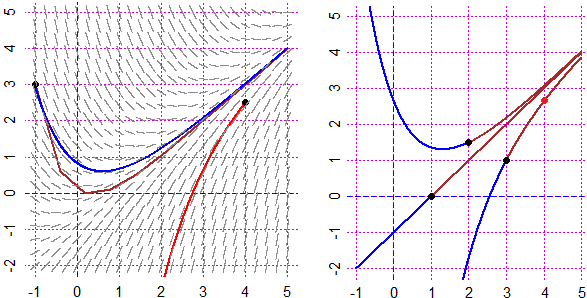 # soledifv(x0,y0, p,N) gives the value of y(p) approximated with N steps
P=soledifv(3,1, 4,1e5); P; P=soledifv(3,1, 4,1e6); P
# 2.632122 2.632121
POINT(p,P, "red") # The red point in the picture
# soledifp(x0,y0,xf,N,col) tracks only N + 1 points without linking them
Plane(-1,5, -2,5)
soledifp(-1,3, 5, 10, "black")
Plane(-1,5, -2,5)
soledif(-1,3, 5, 10, "red")
soledifp(-1,3, 5, 10, "black")
# soledifv(x0,y0, p,N) gives the value of y(p) approximated with N steps
P=soledifv(3,1, 4,1e5); P; P=soledifv(3,1, 4,1e6); P
# 2.632122 2.632121
POINT(p,P, "red") # The red point in the picture
# soledifp(x0,y0,xf,N,col) tracks only N + 1 points without linking them
Plane(-1,5, -2,5)
soledifp(-1,3, 5, 10, "black")
Plane(-1,5, -2,5)
soledif(-1,3, 5, 10, "red")
soledifp(-1,3, 5, 10, "black")
 # In this case (y'=x-y) I know how to solve the equation; the solution is:
f = function(x) x-1+(C+1)*exp(-x)
#
# The solution such that f(3)=1:
# f(3) = 1 implies 2+(C+1)*exp(-3) = 1, C = -1/exp(-3)-1
C = -1/exp(-3)-1
# I can find the value found before:
f(4)
# 2.632121 OK
# If I want I can compare the graphs of the two solutions
Plane(-1,5, -2,5)
POINT(3,1,"black"); soledif(3,1, 5, 1e4, "brown")
graph1(f, -1,5, "blue")
# In this case (y'=x-y) I know how to solve the equation; the solution is:
f = function(x) x-1+(C+1)*exp(-x)
#
# The solution such that f(3)=1:
# f(3) = 1 implies 2+(C+1)*exp(-3) = 1, C = -1/exp(-3)-1
C = -1/exp(-3)-1
# I can find the value found before:
f(4)
# 2.632121 OK
# If I want I can compare the graphs of the two solutions
Plane(-1,5, -2,5)
POINT(3,1,"black"); soledif(3,1, 5, 1e4, "brown")
graph1(f, -1,5, "blue")
 # I can find the solution with WolframAlpha:
# y'(x) = x-y(x), y(3) = 1, y(4) gives 3-1/exp(1) (= 2.632121)
# Another example: y'(x) = 3·y2/3(x)
Dy = function(x,y) 3*(y^2)^(1/3)
Plane(-2,2, -3,3)
diredif(-2,2, -3,3, 20,20)
soledif(1,1, 2, 1e4, "seagreen")
soledif(1,1, -2, 1e4, "seagreen")
soledif(0,0, 2, 1e4, "blue")
soledif(0,0, -2, 1e4, "brown")
soledif(-2,-1, -1, 1e4, "brown")
# I can find the solution with WolframAlpha:
# y'(x) = x-y(x), y(3) = 1, y(4) gives 3-1/exp(1) (= 2.632121)
# Another example: y'(x) = 3·y2/3(x)
Dy = function(x,y) 3*(y^2)^(1/3)
Plane(-2,2, -3,3)
diredif(-2,2, -3,3, 20,20)
soledif(1,1, 2, 1e4, "seagreen")
soledif(1,1, -2, 1e4, "seagreen")
soledif(0,0, 2, 1e4, "blue")
soledif(0,0, -2, 1e4, "brown")
soledif(-2,-1, -1, 1e4, "brown")
 # It is easy verify that y(x) = x3 is a solution such that y(1)=1, but this is not the
# only solution! (WolframAlpha gives only this solution!).
# This example shows how useful it is to trace the directional field.
# A third example: y'(x) = x/y(x) such that y(-3)=2; we want find the value of y(-1.5).
Dy = function(x,y) x/y
Plane(-3,1, -2,2); diredif(-3,1, -2,2, 22,22)
POINT(-3,2, "black")
# It is easy verify that y(x) = x3 is a solution such that y(1)=1, but this is not the
# only solution! (WolframAlpha gives only this solution!).
# This example shows how useful it is to trace the directional field.
# A third example: y'(x) = x/y(x) such that y(-3)=2; we want find the value of y(-1.5).
Dy = function(x,y) x/y
Plane(-3,1, -2,2); diredif(-3,1, -2,2, 22,22)
POINT(-3,2, "black")

 # From the directional field (picture on the left) I can deduce that there is no solution.
# Let's face the problem.
soledif(-3,2, -1.5, 1e5, "seagreen")
# I obtain the green graph (picture on the right); and if I look for the value of the
# solution I find:
soledifv(-3,2, -1.5, 1e5)
# -2.525611 ?!?
# I can use soledifvc that prints the coordinate values of the first four couples of
# points where the slope of the approximate curve-solution changes the sign:
soledifvc(-3,2, -1.5, 1e6)
# -2.236062 -0.00046688 -2.23606 0.006717179
# -2.23606 0.006717179 -2.236059 0.006217848
# -2.236048 -0.0006352839 -2.236047 0.00464436
# -2.236047 0.00464436 -2.236046 0.003922179
# I can improve the approximation of the value:
soledifvc(-3,2, -2.23, 1e6)
# -2.236065 -0.001458657 -2.236064 -0.0002782769
POINT(-2.236,0, "brown")
# Another question. If there are some points where the equation is non defined, it may
# happen that they are not identified by the program.
# An example with the same equation:
PLANE(-3,3, -3,3)
diredif(-3,3, -3,3, 20,20)
soledif(-3,3, 3, 1e4, "brown")
soledif(-3,-3, 3, 1001, "blue")
# From the directional field (picture on the left) I can deduce that there is no solution.
# Let's face the problem.
soledif(-3,2, -1.5, 1e5, "seagreen")
# I obtain the green graph (picture on the right); and if I look for the value of the
# solution I find:
soledifv(-3,2, -1.5, 1e5)
# -2.525611 ?!?
# I can use soledifvc that prints the coordinate values of the first four couples of
# points where the slope of the approximate curve-solution changes the sign:
soledifvc(-3,2, -1.5, 1e6)
# -2.236062 -0.00046688 -2.23606 0.006717179
# -2.23606 0.006717179 -2.236059 0.006217848
# -2.236048 -0.0006352839 -2.236047 0.00464436
# -2.236047 0.00464436 -2.236046 0.003922179
# I can improve the approximation of the value:
soledifvc(-3,2, -2.23, 1e6)
# -2.236065 -0.001458657 -2.236064 -0.0002782769
POINT(-2.236,0, "brown")
# Another question. If there are some points where the equation is non defined, it may
# happen that they are not identified by the program.
# An example with the same equation:
PLANE(-3,3, -3,3)
diredif(-3,3, -3,3, 20,20)
soledif(-3,3, 3, 1e4, "brown")
soledif(-3,-3, 3, 1001, "blue")
 # It may happen that the program overrides x=0 where the equation is not defined.
# A fourth example: y'(x) = (x+y(x))/(x-y(x)) such that y(-2)=1.
Dy = function(x,y) (x+y)/(x-y)
BF=2.7; HF=2.7; Plane(-3,3, -3,3)
diredif(-3,3, -3,3, 20,20)
soledif(-2,1, -3, 1e5, "red")
soledif(-2,1, 3, 1e5, "red")
# It may happen that the program overrides x=0 where the equation is not defined.
# A fourth example: y'(x) = (x+y(x))/(x-y(x)) such that y(-2)=1.
Dy = function(x,y) (x+y)/(x-y)
BF=2.7; HF=2.7; Plane(-3,3, -3,3)
diredif(-3,3, -3,3, 20,20)
soledif(-2,1, -3, 1e5, "red")
soledif(-2,1, 3, 1e5, "red")
 BF=2.7; HF=2.7; Plane(-3,3, -3,3)
soledif(-2,1, -3, 1e5, "red")
soledifvc(-2,1, 3, 1e6)
# -1.146135 1.146135 -1.14613 1.146135
# 0.238275 0.2370324 0.23828 0.238945
# 0.23828 0.238945 0.238285 0.2353571
# 0.238285 0.2353571 0.23829 0.236166
# The first point where the slope changes the sign is a maximum point
soledif(-2,1, 0.2384, 1e5, "red")
POINT(-1.146,1.146, "brown"); POINT(0.2384,0.2345, "blue")
# A fifth example: integral curves of y'(x) + x*y(x)^2/(1+x^2*y(x)) = 0
Dy = function(x,y) -x*y^2/(1+x^2*y)
BF=5; HF=4; Plane(-2.5,2.5, -4,3)
diredif(-2.5,2.5, -4,3, 21,21)
BF=2.7; HF=2.7; Plane(-3,3, -3,3)
soledif(-2,1, -3, 1e5, "red")
soledifvc(-2,1, 3, 1e6)
# -1.146135 1.146135 -1.14613 1.146135
# 0.238275 0.2370324 0.23828 0.238945
# 0.23828 0.238945 0.238285 0.2353571
# 0.238285 0.2353571 0.23829 0.236166
# The first point where the slope changes the sign is a maximum point
soledif(-2,1, 0.2384, 1e5, "red")
POINT(-1.146,1.146, "brown"); POINT(0.2384,0.2345, "blue")
# A fifth example: integral curves of y'(x) + x*y(x)^2/(1+x^2*y(x)) = 0
Dy = function(x,y) -x*y^2/(1+x^2*y)
BF=5; HF=4; Plane(-2.5,2.5, -4,3)
diredif(-2.5,2.5, -4,3, 21,21)
 # through the point (0,2)
soledif(0,2, -3, 1e5, "brown"); soledif(0,2, 3, 1e5, "brown")
soledif(0,1, 3, 1e5, "brown"); soledif(0,1, -3, 1e5, "brown")
# through the point (0,-1)
soledifvc(0,-1, -3, 1e6)
# 0 -1 -3e-06 -1
# -0.707118 -2.00314 -0.707121 -1.997825
# -0.707121 -1.997825 -0.707124 -2.005909
# -0.707124 -2.005909 -0.707127 -2.003067
soledif(0,-1, -0.70711, 1e5, "seagreen"); soledif(0,-1, 0.70711, 1e5, "seagreen")
soledif(-0.7073, -2, -0.1, 1e5, "seagreen"); soledif(0.7073, -2, 0.1, 1e5, "seagreen")
# through the point (0,-1/2)
soledifvc(0,-0.5, -3, 1e6)
# 0 -0.5 -3e-06 -0.5
# -1.000011 -1.000668 -1.000014 -0.9963146
# -1.000014 -0.9963146 -1.000017 -0.9971288
# -1.000026 -1.031578 -1.000029 -1.031477
soledif(0,-1/2, -1, 1e5, "seagreen"); soledif(0,-1/2, 1, 1e5, "seagreen")
soledif(-1.0001, -1.0001, -0.5, 1e5, "seagreen"); soledif(1.0001, -1.0001, 0.5, 1e5, "seagreen")
# through the points (-2,-1), (2,-1)
soledif(-2,-1, -3, 1e5, "blue"); soledif(-2,-1, -0.1, 1e5, "blue")
soledif(2,-1, 3, 1e5, "blue"); soledif(2,-1, 0.1, 1e5, "blue")
# Of course, the simplest differential equations are indefinite integrals, which can be
# studied with simpler methods (see). To trace the directional field it is useful to
# solve other simple differential equations, ot to better understand the solution. An
# example. The differential model f'(x) = f(x) [that is the differential equation y' =
# y] is easy to solve: I know that y=exp(x) is a solution, and that [because Dx(k*f(x))
# = k*Dxf(x)] y(x) = k*exp(x) is also a solution (for every number k). Let's check.
Dy = function(x,y) y
Plane(-2,2, -5,5); diredif(-2,2, -5,5, 15,15)
soledif(0,1, 2, 1e5, "brown"); soledif(0,1, -2, 1e5, "brown")
soledif(-0.5,-2, 2, 1e5, "seagreen"); soledif(-0.5,-2, -2, 1e5, "seagreen")
# Solving the differential equation:
# k*exp(1)=-2 => k=-2/exp(1)
g=function(x) -2/exp(1)*exp(x); POINT(1,-2,"brown")
graph1(g, -2,2, "black")
# through the point (0,2)
soledif(0,2, -3, 1e5, "brown"); soledif(0,2, 3, 1e5, "brown")
soledif(0,1, 3, 1e5, "brown"); soledif(0,1, -3, 1e5, "brown")
# through the point (0,-1)
soledifvc(0,-1, -3, 1e6)
# 0 -1 -3e-06 -1
# -0.707118 -2.00314 -0.707121 -1.997825
# -0.707121 -1.997825 -0.707124 -2.005909
# -0.707124 -2.005909 -0.707127 -2.003067
soledif(0,-1, -0.70711, 1e5, "seagreen"); soledif(0,-1, 0.70711, 1e5, "seagreen")
soledif(-0.7073, -2, -0.1, 1e5, "seagreen"); soledif(0.7073, -2, 0.1, 1e5, "seagreen")
# through the point (0,-1/2)
soledifvc(0,-0.5, -3, 1e6)
# 0 -0.5 -3e-06 -0.5
# -1.000011 -1.000668 -1.000014 -0.9963146
# -1.000014 -0.9963146 -1.000017 -0.9971288
# -1.000026 -1.031578 -1.000029 -1.031477
soledif(0,-1/2, -1, 1e5, "seagreen"); soledif(0,-1/2, 1, 1e5, "seagreen")
soledif(-1.0001, -1.0001, -0.5, 1e5, "seagreen"); soledif(1.0001, -1.0001, 0.5, 1e5, "seagreen")
# through the points (-2,-1), (2,-1)
soledif(-2,-1, -3, 1e5, "blue"); soledif(-2,-1, -0.1, 1e5, "blue")
soledif(2,-1, 3, 1e5, "blue"); soledif(2,-1, 0.1, 1e5, "blue")
# Of course, the simplest differential equations are indefinite integrals, which can be
# studied with simpler methods (see). To trace the directional field it is useful to
# solve other simple differential equations, ot to better understand the solution. An
# example. The differential model f'(x) = f(x) [that is the differential equation y' =
# y] is easy to solve: I know that y=exp(x) is a solution, and that [because Dx(k*f(x))
# = k*Dxf(x)] y(x) = k*exp(x) is also a solution (for every number k). Let's check.
Dy = function(x,y) y
Plane(-2,2, -5,5); diredif(-2,2, -5,5, 15,15)
soledif(0,1, 2, 1e5, "brown"); soledif(0,1, -2, 1e5, "brown")
soledif(-0.5,-2, 2, 1e5, "seagreen"); soledif(-0.5,-2, -2, 1e5, "seagreen")
# Solving the differential equation:
# k*exp(1)=-2 => k=-2/exp(1)
g=function(x) -2/exp(1)*exp(x); POINT(1,-2,"brown")
graph1(g, -2,2, "black")
 #
#  A problem:
# A run-down condenser has capitance C = 80 μF and is connected to a battery of 45 V
# with a resistor of resistance R = 500 Ω. What is the final charge on the condenser?
V=45; C=80*10^-6; R=500 # y is Q (= C*V); Q(0)=0 is the initial condition
Dy = function(t,y) (V-y/C)/R
# Try looking for the solution with a particular graphic scale.
Plane(0,10, 0,1); soledif1(0,0, 10, 1e5, "blue")
A problem:
# A run-down condenser has capitance C = 80 μF and is connected to a battery of 45 V
# with a resistor of resistance R = 500 Ω. What is the final charge on the condenser?
V=45; C=80*10^-6; R=500 # y is Q (= C*V); Q(0)=0 is the initial condition
Dy = function(t,y) (V-y/C)/R
# Try looking for the solution with a particular graphic scale.
Plane(0,10, 0,1); soledif1(0,0, 10, 1e5, "blue")
 # Then, based on the results, I modify it.
Plane(0,10, 0,0.05); soledif1(0,0, 10, 1e5, "blue")
# I modify it.
Plane(0,0.35, 0,0.004); soledif1(0,0, 0.35, 1e5, "blue")
# I look for the limit (from 0 to 0.35 or - better - from 0 to 1)
soledifv(0,0, 1, 1e5)
# 0.0036
coldash="brown"; segm(-1,0.0036, 0.4, 0.0036, 0)
abovex("t"); abovey("Q")
# Then, based on the results, I modify it.
Plane(0,10, 0,0.05); soledif1(0,0, 10, 1e5, "blue")
# I modify it.
Plane(0,0.35, 0,0.004); soledif1(0,0, 0.35, 1e5, "blue")
# I look for the limit (from 0 to 0.35 or - better - from 0 to 1)
soledifv(0,0, 1, 1e5)
# 0.0036
coldash="brown"; segm(-1,0.0036, 0.4, 0.0036, 0)
abovex("t"); abovey("Q")
 # It is not difficult to solve this equation "by hand".
# Let's see how to solve it with Wolfram Alpha
# I put Q(t)/C + R*dQ(t)/dt = V, Q(0)=0
# [or dy(t)/dt = (V-y(t)/C)/R, y(0)=0 ]
# I obtain: Q(t) = C*V*(1-exp(-t/(C*R)))
# Verification:
F = function(t) C*V*( 1-exp(-t/(C*R)) ); graph1(F, 0,0.35, "brown")
# I get a graph that overlaps with the previous one!
# We can verify the solutions of partial differential equations. One example.
f = function(x,y) log(x^2+y^2)
# It is a solution of ∂/∂x ∂/∂x f(x,y) + ∂/∂y ∂/∂y f(x,y) = 0
deriv2(f,"x"); deriv2(f,"y")
# 2/(x^2 + y^2) - 2 * x * (2 * x)/(x^2 + y^2)^2 A
# 2/(x^2 + y^2) - 2 * y * (2 * y)/(x^2 + y^2)^2 B
# It is easy to check algebraically that A+B = 0. Let's check it numerically:
dxxf = function(x,y) eval(deriv2(f,"x")); dyyf = function(x,y) eval(deriv2(f,"y"))
g = function(x,y) dxxf(x,y)+dyyf(x,y)
x=runif(4, 0,20); y=runif(4, 0,20); g(x,y)
# -4.336809e-19 0.000000e+00 -8.673617e-19 1.734723e-18 OK: practically 0
# Other solutions, for any k:
f = function(x,y) exp(k*x)*cos(k*y) # I take for example:
k = 3/7
deriv2(f,"x"); deriv2(f,"y")
# exp(k * x) * k * k * cos(k * y) A
# -(exp(k * x) * (cos(k * y) * k * k)) B
# Numerical verification (instead of the algebraic one) that A + B = 0:
dxxf = function(x,y) eval(deriv2(f,"x")); dyyf = function(x,y) eval(deriv2(f,"y"))
g = function(x,y) dxxf(x,y)+dyyf(x,y)
x=runif(4, 0,20); y=runif(4, 0,20); g(x,y)
# -2.842171e-14 5.551115e-17 2.842171e-14 0.000000e+00 OK: practically 0
# For second-order differential equations see here.
Other examples of use
# It is not difficult to solve this equation "by hand".
# Let's see how to solve it with Wolfram Alpha
# I put Q(t)/C + R*dQ(t)/dt = V, Q(0)=0
# [or dy(t)/dt = (V-y(t)/C)/R, y(0)=0 ]
# I obtain: Q(t) = C*V*(1-exp(-t/(C*R)))
# Verification:
F = function(t) C*V*( 1-exp(-t/(C*R)) ); graph1(F, 0,0.35, "brown")
# I get a graph that overlaps with the previous one!
# We can verify the solutions of partial differential equations. One example.
f = function(x,y) log(x^2+y^2)
# It is a solution of ∂/∂x ∂/∂x f(x,y) + ∂/∂y ∂/∂y f(x,y) = 0
deriv2(f,"x"); deriv2(f,"y")
# 2/(x^2 + y^2) - 2 * x * (2 * x)/(x^2 + y^2)^2 A
# 2/(x^2 + y^2) - 2 * y * (2 * y)/(x^2 + y^2)^2 B
# It is easy to check algebraically that A+B = 0. Let's check it numerically:
dxxf = function(x,y) eval(deriv2(f,"x")); dyyf = function(x,y) eval(deriv2(f,"y"))
g = function(x,y) dxxf(x,y)+dyyf(x,y)
x=runif(4, 0,20); y=runif(4, 0,20); g(x,y)
# -4.336809e-19 0.000000e+00 -8.673617e-19 1.734723e-18 OK: practically 0
# Other solutions, for any k:
f = function(x,y) exp(k*x)*cos(k*y) # I take for example:
k = 3/7
deriv2(f,"x"); deriv2(f,"y")
# exp(k * x) * k * k * cos(k * y) A
# -(exp(k * x) * (cos(k * y) * k * k)) B
# Numerical verification (instead of the algebraic one) that A + B = 0:
dxxf = function(x,y) eval(deriv2(f,"x")); dyyf = function(x,y) eval(deriv2(f,"y"))
g = function(x,y) dxxf(x,y)+dyyf(x,y)
x=runif(4, 0,20); y=runif(4, 0,20); g(x,y)
# -2.842171e-14 5.551115e-17 2.842171e-14 0.000000e+00 OK: practically 0
# For second-order differential equations see here.
Other examples of use