source("http://macosa.dima.unige.it/r.R") # If I have not already loaded the library
---------- ---------- ---------- ---------- ---------- ---------- ---------- ----------
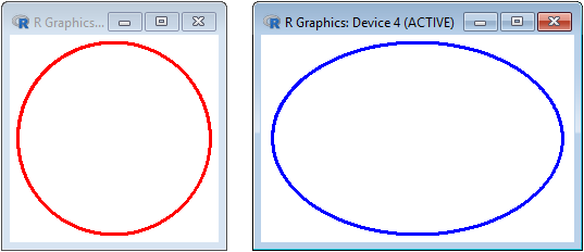
S 16 Windows without the margins
# boxW opens a new coordinate system with nothing, no grid or axes, filling the window
# (without the space usually used for the coordinates). BOXW does the same using a
# monometric scale. I can use these commands (using 0,0,0,0 as input) even before
# the "persp" command to reduce whitespace.
# If I want to add grids I can use, for example, gridh and gridv (see), or BOX().
BF=2; HF=2; BOXW(-1,1, -1,1)
circle(0,0, 1, "red")
BF=3; HF=2; boxW(-1,1, -1,1)
circle(0,0, 1, "blue")
 # boxWW and BOXWW leave a bit of space above and on the right:
BF=3; HF=2; boxWW(-1,1, -1,1); circle(0,0, 1, "blue"); abovex("xxxxx"); abovey("yyyyy")
BF=2; HF=2; BOXWW(-1,1, -1,1); circle(0,0, 1, "red"); abovex("xxxxx"); abovey("yyyyy")
# boxWW and BOXWW leave a bit of space above and on the right:
BF=3; HF=2; boxWW(-1,1, -1,1); circle(0,0, 1, "blue"); abovex("xxxxx"); abovey("yyyyy")
BF=2; HF=2; BOXWW(-1,1, -1,1); circle(0,0, 1, "red"); abovex("xxxxx"); abovey("yyyyy")

 # boxww and BOXww leave a bit of space under and on the left:
BF=3; HF=2; boxww(-1,1, -1,1); circle(0,0, 1, "blue"); underx("xxxxx"); undery("yyyyy")
BF=2; HF=2; BOXww(-1,1, -1,1); circle(0,0, 1, "red"); underx("xxxxx"); undery("yyyyy")
# boxww and BOXww leave a bit of space under and on the left:
BF=3; HF=2; boxww(-1,1, -1,1); circle(0,0, 1, "blue"); underx("xxxxx"); undery("yyyyy")
BF=2; HF=2; BOXww(-1,1, -1,1); circle(0,0, 1, "red"); underx("xxxxx"); undery("yyyyy")


 # You can employ boxWW to use non-decimal scale (see here for the above picture).
# house
A <- c(1,4, 5,4, 5,0, 1,0, 1,4, 3,5, 5,4); xTab(A); yTab(A)
# [1] 1 5 5 1 1 3 5
# [1] 4 4 0 0 4 5 4
BF=2.5; HF=2.5
PLANE(0,6, 0,6); polyline(xTab(A), yTab(A), "red")
BOXW(0,6, 0,6); polyline(xTab(A), yTab(A), "red")
BOXW(0,6, 0,6); polyC(xTab(A), yTab(A), "yellow")
BOX()
# You can employ boxWW to use non-decimal scale (see here for the above picture).
# house
A <- c(1,4, 5,4, 5,0, 1,0, 1,4, 3,5, 5,4); xTab(A); yTab(A)
# [1] 1 5 5 1 1 3 5
# [1] 4 4 0 0 4 5 4
BF=2.5; HF=2.5
PLANE(0,6, 0,6); polyline(xTab(A), yTab(A), "red")
BOXW(0,6, 0,6); polyline(xTab(A), yTab(A), "red")
BOXW(0,6, 0,6); polyC(xTab(A), yTab(A), "yellow")
BOX()
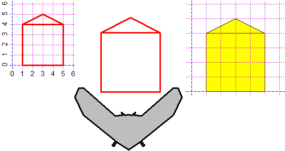 # spider
P <- c(
0, 1.05, 0.1,1.05, 0.35,1, 0.8,1.3, 0.6,0.95,
1.5,0.9, 5,4, 5.55,4, 6,3, 5,1,
1.45,-1.9, 1.8,-2.4, 1.6,-2.5, 1.35,-2, 0,-2.9,
-1.35,-2, -1.6,-2.5, -1.8,-2.4, -1.45,-1.9, -5,1,
-6,3, -5.55,4, -5,4, -1.5,0.9, -0.6,0.95,
-0.8,1.3, -0.35,1, -0.1,1.05, 0,1.05 )
X <- xTab(P); Y <- yTab(P)
BOXW(-6,6, -6,6); polyC(X, Y, "grey")
polyline(X, Y, "black")
# type BOX() to see the grid
Other examples of use
# spider
P <- c(
0, 1.05, 0.1,1.05, 0.35,1, 0.8,1.3, 0.6,0.95,
1.5,0.9, 5,4, 5.55,4, 6,3, 5,1,
1.45,-1.9, 1.8,-2.4, 1.6,-2.5, 1.35,-2, 0,-2.9,
-1.35,-2, -1.6,-2.5, -1.8,-2.4, -1.45,-1.9, -5,1,
-6,3, -5.55,4, -5,4, -1.5,0.9, -0.6,0.95,
-0.8,1.3, -0.35,1, -0.1,1.05, 0,1.05 )
X <- xTab(P); Y <- yTab(P)
BOXW(-6,6, -6,6); polyC(X, Y, "grey")
polyline(X, Y, "black")
# type BOX() to see the grid
Other examples of use